Trajectory and Pseudotime Analysis

scVelo Tutorial for Trajectory Analysis
Palantir Tutorial for Trajectory and Pseudotime Analysis
MAGIC for Denoising and Smoothing Gene Expression
CellRank Tutorial for Trajectory Analysis
Gene Expression Dynamics Along Differentiation Trajectories
Slingshot Tutorial for Pseudotime Analysis
Integration of Seurat with Python Tools

Analyzing Single-Cell Trajectories with scVelo

scVelo is a widely used tool for trajectory analysis that leverages spliced and unspliced RNA information, as calculated by Velocyto, to predict the direction of cell differentiation. For more information, see scVelo’s documentation. SeuratExtend includes a series of functions that allow you to easily run everything in R. In this tutorial, we use an example dataset (pbmc10k_10X) downloaded from the 10X Genomics website, focusing on a small subset of myeloid cells for simplicity.

Downloading Example Data

First, we need to download the example data, including a small Seurat object and a corresponding small loom file generated by Velocyto. These files are stored on Zenodo:

library(Seurat)
library(SeuratExtend)

# Download the example Seurat Object
mye_small <- readRDS(url("https://zenodo.org/records/10944066/files/pbmc10k_mye_small_velocyto.rds", "rb"))

# Download the example velocyto loom file
loom_path <- file.path(tempdir(), "pbmc10k_mye_small.loom")
download.file("https://zenodo.org/records/10944066/files/pbmc10k_mye_small.loom", 
              loom_path,
              mode = "wb")  # Use binary mode for Windows compatibility

Note:

When downloading loom files (which are HDF5-based binary files) on Windows, it’s essential to use mode = "wb" in the download.file() function. This prevents Windows from modifying line endings in the binary file, which would corrupt the HDF5 format. Mac and Linux users don’t require this parameter, but including it is harmless.
To save disk space, the data downloaded for this tutorial is stored in the temporary folder and will be automatically deleted after the R session is closed. If you wish to permanently retain the tutorial files, please manually change the storage location to your working directory.

Preparing Data for scVelo

scVelo requires an AnnData object from Python’s Scanpy library for its analyses. SeuratExtend makes this process seamless by integrating a Seurat object and a velocyto loom file into a new AnnData object, serving as a bridge between R and Python.

Note: If this is your first time running Python-related functions (scVelo, Palantir, etc.) in SeuratExtend, it will prompt you to install a conda environment named “seuratextend”. This environment automatically installs all required Python packages. It is currently supported and tested on Windows, Intel-based macOS (not Apple Silicon/M1/M2), and Linux (Ubuntu 20.04) systems. Users with Apple Silicon devices who are interested in contributing to the development of M1/M2 support are welcome to reach out via GitHub Issues. More details on managing the Anndata object and Python dependencies are provided here: Integration of Seurat with Python Tools.

# Set up the path for saving the AnnData object in the HDF5 (h5ad) format
if (.Platform$OS.type == "windows") {
    adata_path <- normalizePath(file.path(tempdir(), "mye_small.h5ad"), winslash = "/")
} else {
    adata_path <- file.path(tempdir(), "mye_small.h5ad")
}

# Integrate Seurat Object and velocyto loom information into one AnnData object.
# This object will be stored at the specified path.
scVelo.SeuratToAnndata(
  mye_small, # The downloaded example Seurat object
  filename = adata_path, # Path where the AnnData object will be saved
  velocyto.loompath = loom_path, # Path to the loom file
  prefix = "sample1_", # Prefix for cell IDs in the Seurat object
  postfix = "-1" # Postfix for cell IDs in the Seurat object
)

## Running scvelo 0.3.0 (python 3.10.12) on 2024-11-28 17:07.
## Filtered out 10891 genes that are detected 20 counts (shared).
## Normalized count data: X, spliced, unspliced.
## Extracted 2000 highly variable genes.
## Logarithmized X.
## computing neighbors
##     finished (0:00:04) --> added 
##     'distances' and 'connectivities', weighted adjacency matrices (adata.obsp)
## computing moments based on connectivities
##     finished (0:00:00) --> added 
##     'Ms' and 'Mu', moments of un/spliced abundances (adata.layers)
## computing velocities
##     finished (0:00:00) --> added 
##     'velocity', velocity vectors for each individual cell (adata.layers)
## computing velocity graph (using 1/28 cores)
## WARNING: Unable to create progress bar. Consider installing `tqdm` as `pip install tqdm` and `ipywidgets` as `pip install ipywidgets`,
## or disable the progress bar using `show_progress_bar=False`.
##     finished (0:00:01) --> added 
##     'velocity_graph', sparse matrix with cosine correlations (adata.uns)

Generating scVelo Plots

Now, you’re ready to generate scVelo plots. The default dimension reduction method is typically UMAP, colored by cluster.

scVelo.Plot(color = "cluster", save = "umap1.png", figsize = c(5,4))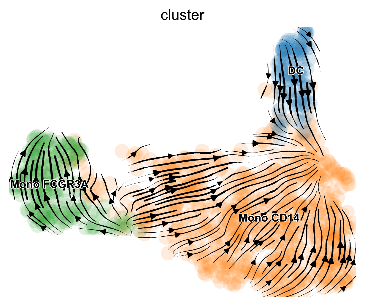

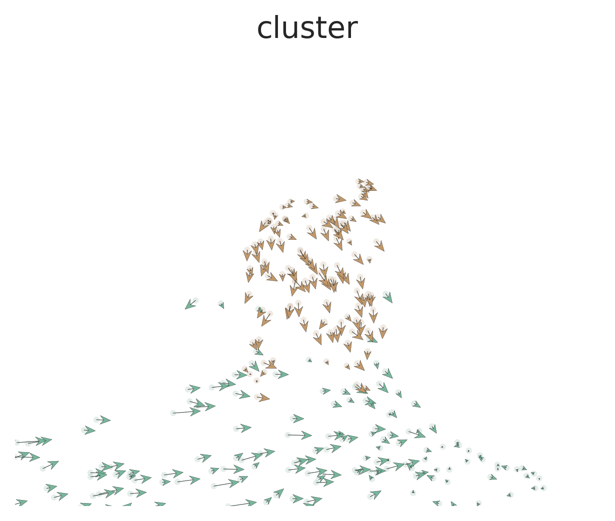
SeuratExtend supports most commonly used parameters for scVelo plots. You can customize the plot style, dimensionality reduction method, color palette, displayed clusters, and more. For more detailed information on customization and advanced features, refer to the function documentation or the official scVelo documentation.

scVelo.Plot(
  style = "scatter",
  color = "cluster",
  groups = c("DC", "Mono CD14"),
  palette = color_pro(3, "light"),
  xlim = c(0, 5), ylim = c(0, 10),
  save = "umap2_specified_area.png",
  figsize = c(5,4)
)

Palantir Tutorial for Trajectory and Pseudotime Analysis

Introduction

Palantir is a Python tool designed for aligning cells along differentiation trajectories, determining cell fate, and calculating pseudotime. SeuratExtend enables these functionalities within R, storing the results in a Seurat object for streamlined analysis.

Downloading Example Data

We will use a subset of myeloid cells from the pbmc10k_10X dataset available on the 10X Genomics website. If you have already loaded the Seurat object, you can skip this step.

library(Seurat)
library(SeuratExtend)

# Download the example Seurat Object
mye_small <- readRDS(url("https://zenodo.org/records/10944066/files/pbmc10k_mye_small_velocyto.rds", "rb"))

Running Diffusion Map

Palantir aligns cells along differentiation trajectories by first calculating the diffusion map. This is done in Python via reticulate, based on pre-calculated dimension reductions in Seurat (e.g., PCA, harmony). The diffusion map (dm) and multiscale space (ms) embeddings are then added back to the Seurat object.

mye_small <- Palantir.RunDM(mye_small)

## Determing nearest neighbor graph...

# View the new dimensional reductions "dm" and "ms" in the Seurat Object:
mye_small@reductions

## $pca
## A dimensional reduction object with key PC_ 
##  Number of dimensions: 50 
##  Number of cells: 1000 
##  Projected dimensional reduction calculated:  FALSE 
##  Jackstraw run: FALSE 
##  Computed using assay: RNA 
## 
## $umap
## A dimensional reduction object with key UMAP_ 
##  Number of dimensions: 2 
##  Number of cells: 1000 
##  Projected dimensional reduction calculated:  FALSE 
##  Jackstraw run: FALSE 
##  Computed using assay: RNA 
## 
## $dm
## A dimensional reduction object with key DM_ 
##  Number of dimensions: 50 
##  Number of cells: 1000 
##  Projected dimensional reduction calculated:  FALSE 
##  Jackstraw run: FALSE 
##  Computed using assay: RNA 
## 
## $ms
## A dimensional reduction object with key MS_ 
##  Number of dimensions: 2 
##  Number of cells: 1000 
##  Projected dimensional reduction calculated:  FALSE 
##  Jackstraw run: FALSE 
##  Computed using assay: RNA

# View the first 2 ms dimensions:
DimPlot2(mye_small, reduction = "ms", group.by = "cluster", label = TRUE)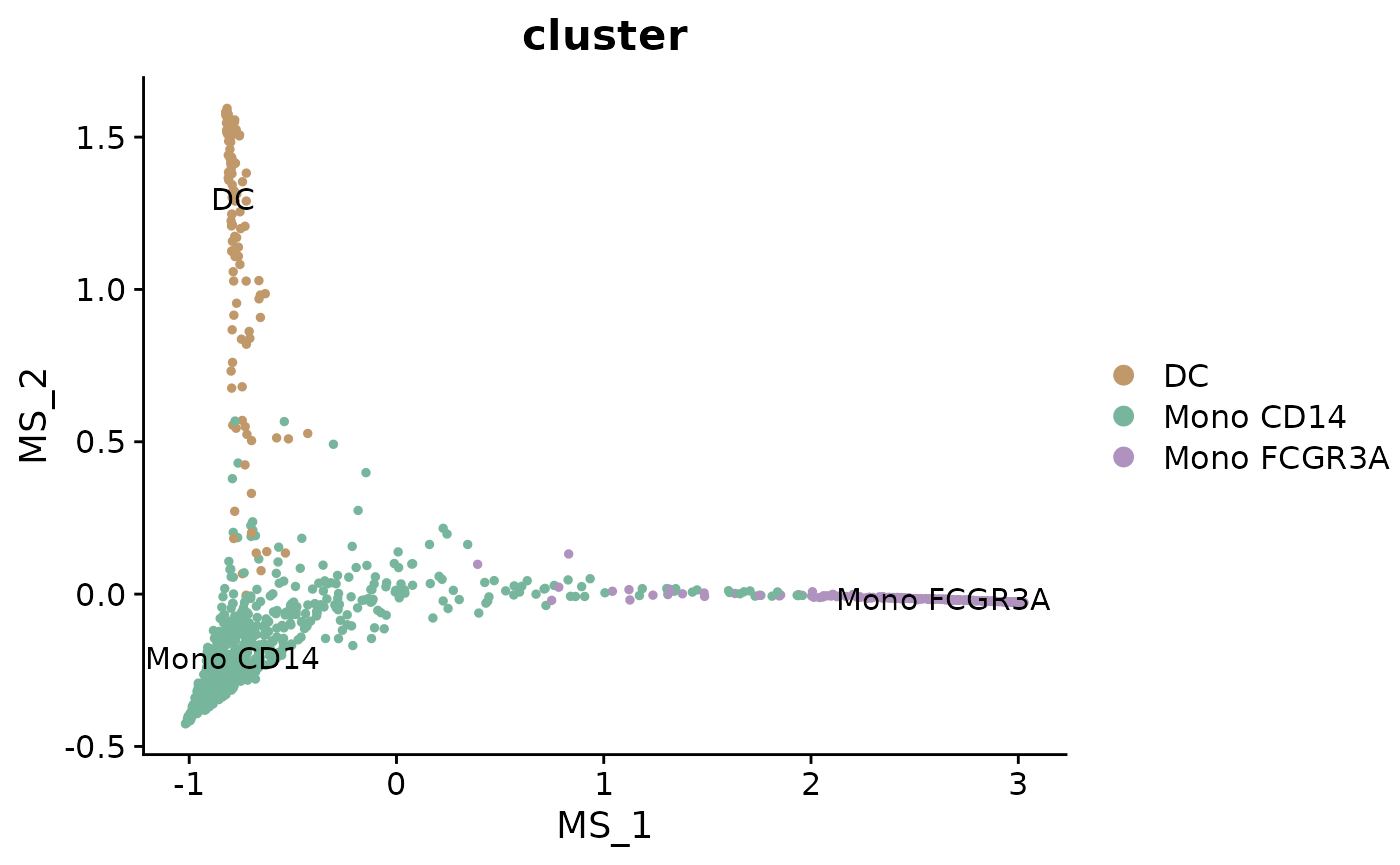

UMAP Based on “ms”

In this simple example, the multiscale space (‘ms’) reduction has only 2 dimensions, which makes additional dimension reduction unnecessary for visualization. However, in more complex datasets, ‘ms’ reductions often yield more dimensions, necessitating further reduction for effective visualization.

For such cases, one can create a new differentiation trajectory space by running UMAP based on the “ms” reduction. This approach allows for a more comprehensible display in a two-dimensional plot, especially when dealing with a higher-dimensional ‘ms’ space. The following code, although not run in this tutorial, illustrates how to implement UMAP on ‘ms’ with hypothetical ten dimensions and visualize the result:

# Assuming 'ms' has 10 dimensions:
# mye_small <- RunUMAP(mye_small, reduction = "ms", dims = 1:10)
# DimPlot2(mye_small, group.by = "cluster", label = TRUE, reduction = "umap")

(Optional) Incorporating Newly Calculated Dimension Reductions into AnnData

If you’ve previously followed the scVelo tutorial, an adata object should already exist in your Python environment. If you wish to incorporate the dimension reductions calculated by Palantir (such as ‘ms’) into this adata and use it for visualization, you can do so with the following commands:

# Add the 'ms' dimension reduction to the existing AnnData object
adata.AddDR(mye_small, dr = "ms", scv.graph = TRUE)

# Generate a plot using the newly added 'ms' dimension reduction
scVelo.Plot(basis = "ms", color = "cluster", save = "umap3_ms.png", figsize = c(5,4))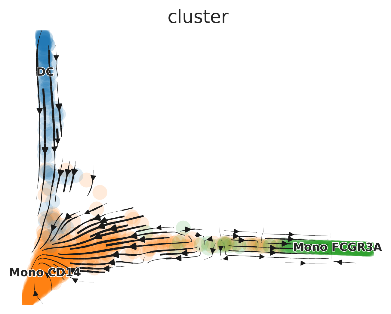

Determining Cell Fates and Calculating Pseudotime

To predict cell fates and calculate pseudotime, You can manually select “start cells” using the CellSelector function.

p <- DimPlot(mye_small, reduction = "ms", group.by = "cluster")
cells <- CellSelector(p)

Then, calculate pseudotime. Results are stored in SeuratObj@misc$Palantir$Pseudotime.

mye_small <- Palantir.Pseudotime(mye_small, start_cell = "sample1_GAGAGGTAGCAGTACG-1")

## Sampling and flocking waypoints...
## Time for determining waypoints: 0.0011072675387064615 minutes
## Determining pseudotime...
## Shortest path distances using 30-nearest neighbor graph...
## Time for shortest paths: 0.10401349465052287 minutes
## Iteratively refining the pseudotime...
## Correlation at iteration 1: 1.0000
## Entropy and branch probabilities...
## Markov chain construction...
## Identification of terminal states...
## Computing fundamental matrix and absorption probabilities...
## Project results to all cells...

ps <- mye_small@misc$Palantir$Pseudotime
head(ps)

##                            Pseudotime   Entropy sample1_AAACCCAAGGCCCAAA.1
## sample1_GAGTCATGTACCCGCA-1  0.0369992 0.6087369                  0.7024933
## sample1_TGGAGGAGTGTATACC-1  0.1307173 0.6093996                  0.7017203
## sample1_CCCGGAAGTTGGCTAT-1  0.1137811 0.6082388                  0.7030721
## sample1_CTGAGGCAGTCAGGGT-1  0.2990304 0.4924385                  0.8056717
## sample1_GCCAACGTCCCGTGTT-1  0.1455877 0.6137009                  0.6966202
## sample1_TCAAGCAGTGTGGTCC-1  0.0759786 0.6087872                  0.7024348
##                            sample1_CCTCTAGGTGAACGGT.1
## sample1_GAGTCATGTACCCGCA-1                  0.2975067
## sample1_TGGAGGAGTGTATACC-1                  0.2982797
## sample1_CCCGGAAGTTGGCTAT-1                  0.2969279
## sample1_CTGAGGCAGTCAGGGT-1                  0.1943283
## sample1_GCCAACGTCCCGTGTT-1                  0.3033798
## sample1_TCAAGCAGTGTGGTCC-1                  0.2975652

# Visualize cell fate on UMAP
colnames(ps)[3:4] <- c("fate1", "fate2")
mye_small@meta.data[,colnames(ps)] <- ps
DimPlot2(mye_small, features = colnames(ps), reduction = "ms", 
         cols = list(Entropy = "D"), theme = NoAxes())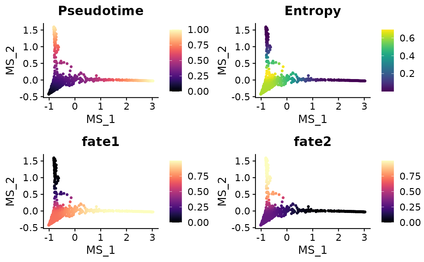

## Loading required package: viridis

## Loading required package: viridisLite

MAGIC for Denoising and Smoothing Gene Expression

Another related tool, MAGIC (Markov Affinity-based Graph Imputation of Cells), denoises and smooths gene expression in scRNA-seq data. Here’s how to run it and observe the differences in gene expression:

mye_small <- Palantir.Magic(mye_small)

## Determing nearest neighbor graph...

## Warning: Layer counts isn't present in the assay object; returning NULL

# Creates a new assay "magic" in the Seurat object
mye_small <- NormalizeData(mye_small)
DimPlot2(mye_small, features = c("CD14", "magic_CD14", "FLT3", "magic_FLT3"), 
         cols = "A", theme = NoAxes())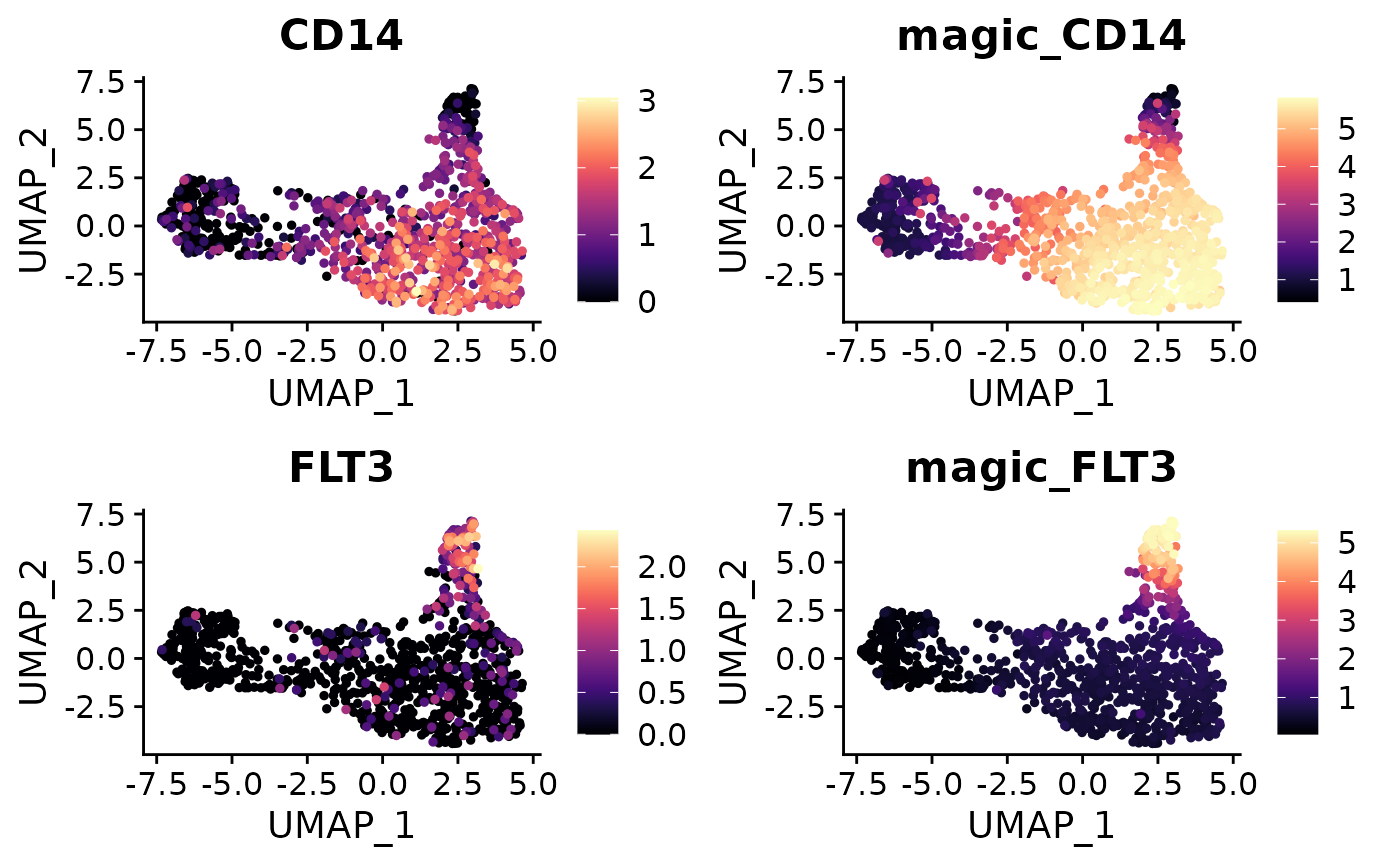

CellRank Tutorial for Trajectory Analysis

Introduction

While scVelo is a powerful tool for predicting differentiation potential, it may sometimes produce arrows pointing opposite the known differentiation trajectory, which is inconsistent with biological knowledge. For more details and examples, visit the CellRank documentation. In such cases, CellRank offers an alternative by utilizing pre-calculated pseudotime to create trajectory plots. However, it’s crucial to ensure that the pseudotime calculation aligns with validated biological knowledge to avoid misuse of the algorithm.

This tutorial assumes you have already completed the tutorials for velocyto and Palantir. We will use CellRank to build trajectory plots, continuing from where those tutorials left off.

Adding Pseudotime to the `adata` Object

First, we add the Pseudotime calculated by Palantir to the adata object. This information is saved in the meta.data of the Seurat Object. We transfer the relevant column from Seurat to adata:

adata.AddMetadata(mye_small, col = colnames(ps))

Running CellRank Kernel

Next, we run the CellRank Kernel to compute the trajectory plots using the previously added Pseudotime information.

Cellrank.Compute(time_key = "Pseudotime")

Generating the Plots

The process for generating plots with CellRank is similar to that used with scVelo.Plot:

# Generate a plot using the 'ms' dimension reduction
Cellrank.Plot(color = "cluster", basis = "ms", save = "umap3_ms_cellrank.png")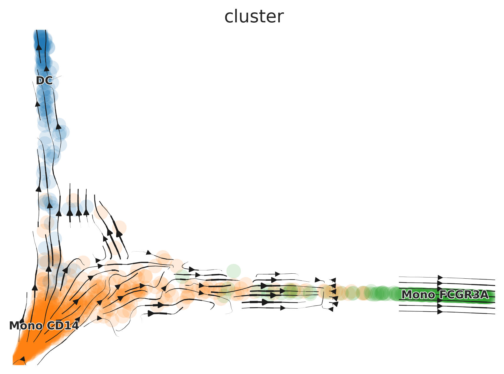

Gene Expression Dynamics Along Differentiation Trajectories]

Visualizing smoothed gene expression along a trajectory offers insightful perspectives on cellular differentiation and development. SeuratExtend introduces two methods for such visualization, leveraging the pseudotime calculated by tools like Palantir.

Gene Trend Curves with Palantir

Assuming you have already executed Palantir.Pseudotime as shown in a previous tutorial, you can create gene trend curves as follows:

library(SeuratExtend)

# Basic gene trend curve visualization
GeneTrendCurve.Palantir(mye_small, features = c("CD14", "FCGR3A"))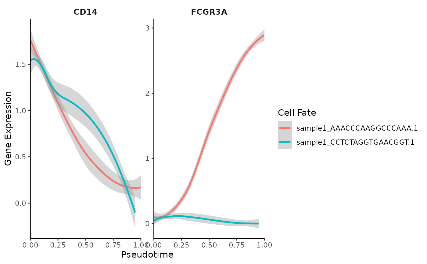

Customizing Gene Trend Curves

You can customize the plots, for instance, by adding points, removing confidence intervals, and renaming cell fates:

# Accessing pseudotime and adjusting fate names
ps <- mye_small@misc$Palantir$Pseudotime
head(ps)

##                            Pseudotime   Entropy sample1_AAACCCAAGGCCCAAA.1
## sample1_GAGTCATGTACCCGCA-1  0.0369992 0.6087369                  0.7024933
## sample1_TGGAGGAGTGTATACC-1  0.1307173 0.6093996                  0.7017203
## sample1_CCCGGAAGTTGGCTAT-1  0.1137811 0.6082388                  0.7030721
## sample1_CTGAGGCAGTCAGGGT-1  0.2990304 0.4924385                  0.8056717
## sample1_GCCAACGTCCCGTGTT-1  0.1455877 0.6137009                  0.6966202
## sample1_TCAAGCAGTGTGGTCC-1  0.0759786 0.6087872                  0.7024348
##                            sample1_CCTCTAGGTGAACGGT.1
## sample1_GAGTCATGTACCCGCA-1                  0.2975067
## sample1_TGGAGGAGTGTATACC-1                  0.2982797
## sample1_CCCGGAAGTTGGCTAT-1                  0.2969279
## sample1_CTGAGGCAGTCAGGGT-1                  0.1943283
## sample1_GCCAACGTCCCGTGTT-1                  0.3033798
## sample1_TCAAGCAGTGTGGTCC-1                  0.2975652

colnames(ps)[3:4] <- c("fate1", "fate2")

# Customized gene trend curve visualization
GeneTrendCurve.Palantir(
  mye_small, 
  pseudotime.data = ps, 
  features = c("CD14", "FCGR3A"),
  point = TRUE, 
  se = FALSE
)

## `geom_smooth()` using method = 'loess' and formula = 'y ~ x'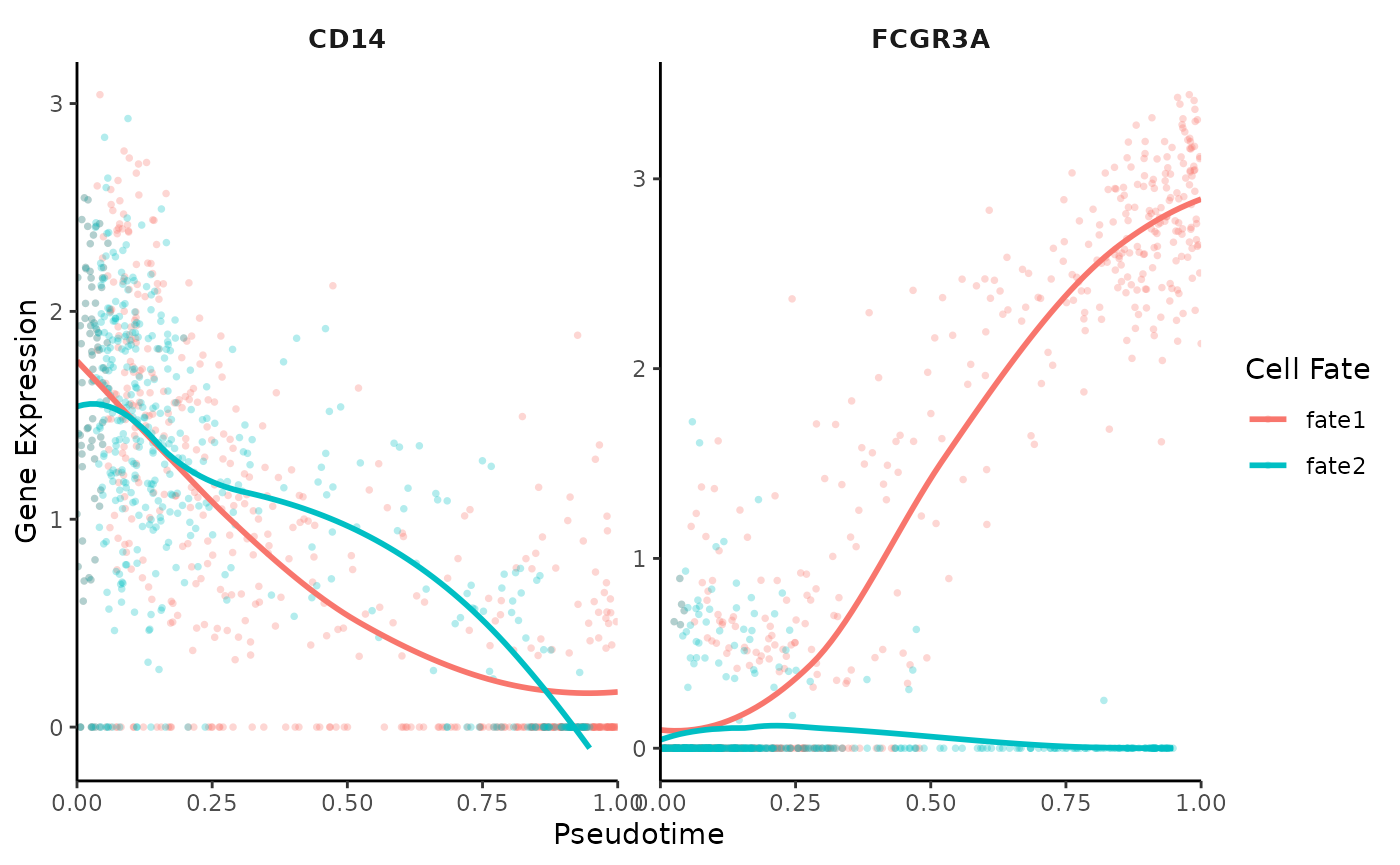

Gene Trend Heatmaps with Palantir

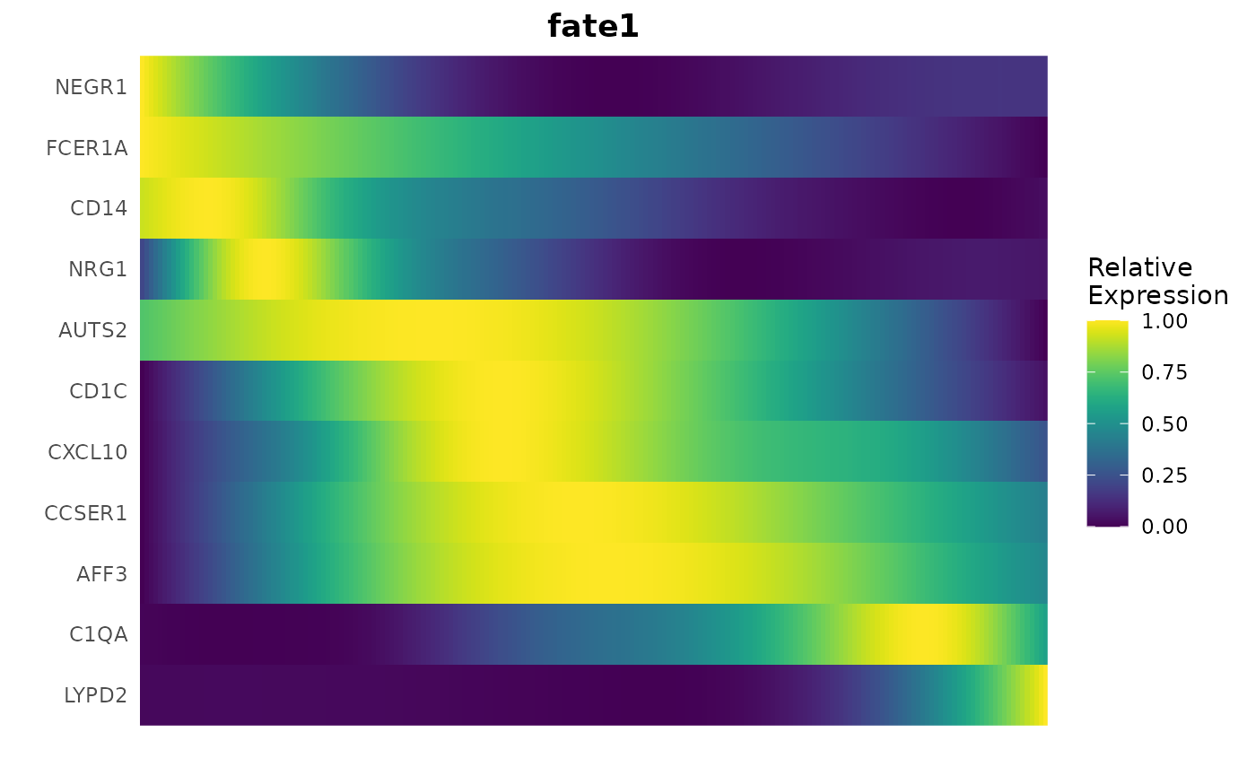
Another powerful method for visualizing gene expression dynamics is through heatmaps, which can illustrate how gene expression changes across pseudotime and for specific lineages:

# Creating a gene trend heatmap
GeneTrendHeatmap.Palantir(
  mye_small, 
  features = c("CD14", VariableFeatures(mye_small)[1:10]), 
  pseudotime.data = ps, 
  magic = FALSE, 
  lineage = "fate1"
)

Slingshot Tutorial for Pseudotime Analysis

Apart from Palantir, Slingshot is another valuable tool for calculating pseudotime, particularly useful for mapping cellular trajectories in single-cell RNA sequencing data.

Running Slingshot

To calculate pseudotime using Slingshot, we start by integrating it with our Seurat object:

library(SeuratExtend)

mye_small <- RunSlingshot(mye_small, group.by = "cluster", start.clus = "Mono CD14")

Accessing Slingshot Output

The Slingshot output is stored within the Seurat object. Let’s extract the pseudotime values and visualize them on the UMAP:

sling <- mye_small@misc$slingshot$PCA$SlingPseudotime
head(sling)

## DataFrame with 6 rows and 2 columns
##                            slingPseudotime_1 slingPseudotime_2
##                                    <numeric>         <numeric>
## sample1_GAGTCATGTACCCGCA-1           12.3665           12.3423
## sample1_TGGAGGAGTGTATACC-1           20.2568           20.3749
## sample1_CCCGGAAGTTGGCTAT-1           19.6071           19.7093
## sample1_CTGAGGCAGTCAGGGT-1           26.1367           28.3753
## sample1_GCCAACGTCCCGTGTT-1           17.0883           17.5357
## sample1_TCAAGCAGTGTGGTCC-1           16.5014           16.4016

mye_small@meta.data[,colnames(sling)] <- as.data.frame(sling)

DimPlot2(mye_small, features = colnames(sling), cols = "C", theme = NoAxes())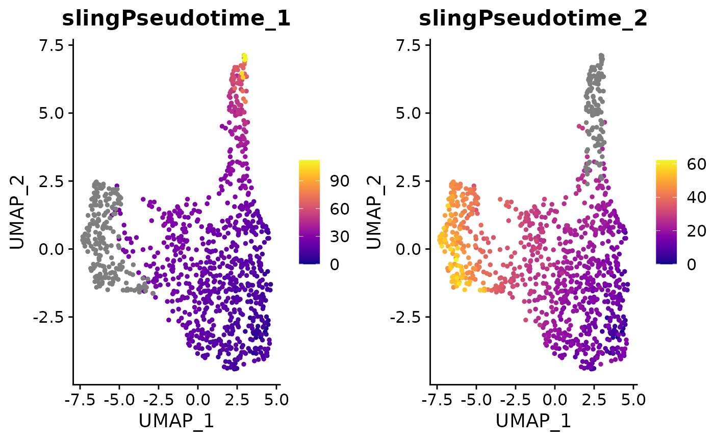

Gene Trend Curves for Slingshot Pseudotime

Similar to Palantir, Slingshot pseudotime allows for the creation of gene trend curves, illustrating the dynamics of gene expression along the computed trajectories:

GeneTrendCurve.Slingshot(mye_small, features = c("CD14", "FCGR3A"))

## `geom_smooth()` using method = 'loess' and formula = 'y ~ x'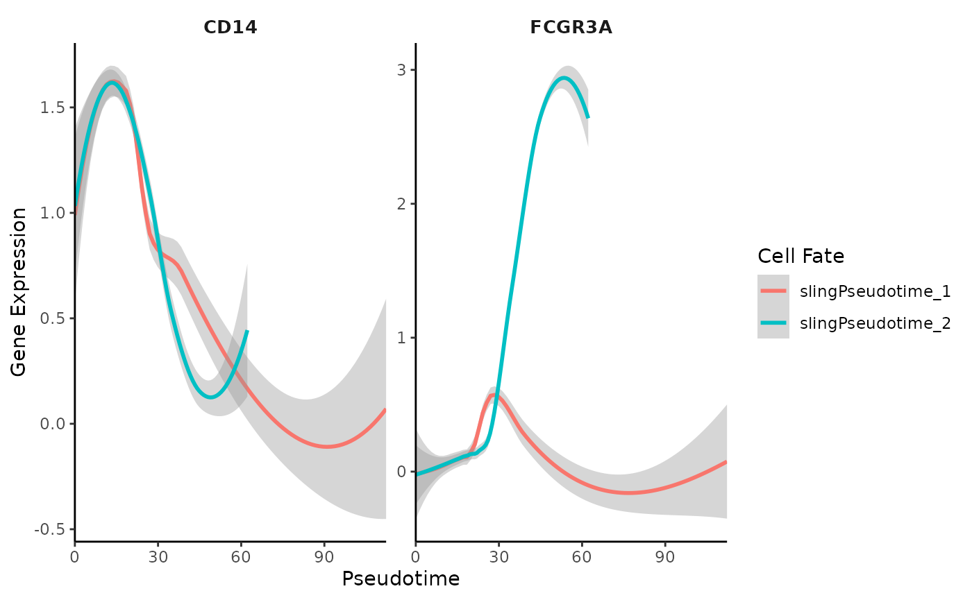

Visualizing Gene Trends with Heatmaps

Additionally, Slingshot pseudotime can be used to generate heatmaps, showcasing the progression of gene expression across different lineages:

GeneTrendHeatmap.Slingshot(
  mye_small, 
  features = c("CD14", VariableFeatures(mye_small)[1:10]), 
  lineage = "slingPseudotime_2"
)

## Using id as id variables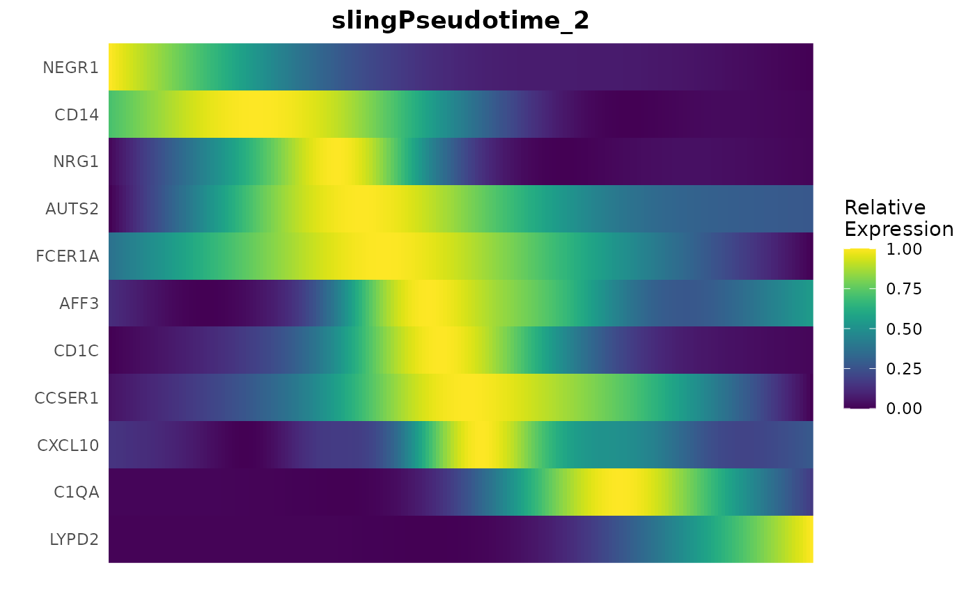

Integration of Seurat with Python Tools

Introduction

SeuratExtend incorporates numerous functions that utilize Python packages such as Scanpy, scVelo, Palantir, and CellRank. This integration facilitates a seamless workflow between Seurat objects and AnnData formats, crucial for leveraging the comprehensive analytical capabilities of both R and Python ecosystems.

To understand the mechanisms behind these functions, it is important to grasp the fundamentals of how Seurat and AnnData communicate. Initially, loom files serve as the intermediary; these h5 format files are widely used for storing scRNA-seq data and are compatible with both R and Python. Tools such as velocyto and SCENIC utilize loom files, which can store gene expression and metadata but have limitations, such as the inability to store dimensional reduction and neighborhood graph information.

In SeuratExtend, the conversion from a Seurat object to an AnnData object does not occur directly. Instead, loom files act as a bridge—first converting Seurat to loom and then from loom to AnnData. The loss of dimensional reduction information during this process is compensated by other related functions within SeuratExtend.

Creating a Conda Environment with All Required Python Packages

If it is your first time running functions related to scVelo, Palantir, or CellRank, you will be automatically prompted to install a Conda environment named “seuratextend”. This environment includes all the Python packages required by SeuratExtend and is managed through reticulate.

Note: Before creating the conda environment, ensure that Git is installed on your system, as it’s required for installing certain Python packages:

Windows: Download and install from Git for Windows
Mac: Install via Homebrew (brew install git) or Xcode Command Line Tools (xcode-select --install)
Linux: Install using your package manager:
- Ubuntu/Debian: sudo apt-get install git
- Fedora: sudo dnf install git
- CentOS/RHEL: sudo yum install git

If you prefer to initiate the conda environment installation step manually, you can easily do so by running:

create_condaenv_seuratextend()

This function automatically detects your operating system and sets up the environment accordingly. It is currently supported and tested on Windows, Intel-based macOS (not Apple Silicon/M1/M2), and Linux (Ubuntu 20.04) systems. Users with Apple Silicon devices who are interested in contributing to the development of M1/M2 support are welcome to reach out via GitHub Issues.

Integrating Seurat with AnnData

In this section, we demonstrate the utility of functions designed to bridge Seurat objects with Python’s AnnData structures, using a small pbmc Seurat object as an example. The process covers conversion to a loom file, importing into AnnData, and appending additional metadata and dimension reduction data.

Converting Seurat Object to Loom

First, we convert a Seurat object to a loom file which can then be used to create an AnnData object:

# Convert Seurat object to loom file and save it locally
pbmc_loom_path <- file.path(tempdir(), "pbmc3k_small.loom")
Seu2Loom(pbmc, filename = pbmc_loom_path, add.normdata = TRUE)

Importing Loom File into AnnData

Next, we import the loom file into an AnnData object, which is handled by Python:

# Load the loom file into an AnnData object
adata.LoadLoom(loompath = pbmc_loom_path)

Viewing AnnData Object

To view the newly created AnnData object, we use reticulate to execute Python code:

# Print the AnnData object details
py_run_string("print(adata)")

## AnnData object with n_obs × n_vars = 500 × 12627
##     obs: 'RNA_snn_res.0.5', 'cluster', 'nCount_RNA', 'nFeature_RNA', 'orig.ident', 'percent.mt', 'seurat_clusters'
##     layers: 'counts'

Adding Dimension Reduction Data

AnnData objects can store more than just gene expression and metadata; here we add dimension reduction data from Seurat:

# Add dimension reduction data from Seurat to AnnData
adata.AddDR(pbmc)
# Print the updated AnnData object
py_run_string("print(adata)")

## AnnData object with n_obs × n_vars = 500 × 12627
##     obs: 'RNA_snn_res.0.5', 'cluster', 'nCount_RNA', 'nFeature_RNA', 'orig.ident', 'percent.mt', 'seurat_clusters'
##     obsm: 'X_pca', 'X_umap'
##     layers: 'counts'

Direct Conversion from Seurat to AnnData

For a streamlined conversion that includes the steps of Seu2Loom(), adata.LoadLoom() and adata.AddDR(), you can use a single function:

# Directly convert Seurat object to AnnData object
Seu2Adata(pbmc)

Updating AnnData with New Metadata

If new metadata columns are added to the Seurat object, they can also be incorporated into the AnnData object:

# Add new metadata column to AnnData
pbmc$cluster2 <- pbmc$cluster
adata.AddMetadata(pbmc, col = "cluster2")
# Print the updated AnnData object
py_run_string("print(adata)")

## AnnData object with n_obs × n_vars = 500 × 12627
##     obs: 'RNA_snn_res.0.5', 'cluster', 'nCount_RNA', 'nFeature_RNA', 'orig.ident', 'percent.mt', 'seurat_clusters', 'cluster2'
##     obsm: 'X_pca', 'X_umap'
##     layers: 'counts'

Saving and Loading AnnData

You can save the AnnData object to a local file for future use:

# Save the AnnData object to a local file
pbmc_adata_path <- file.path(tempdir(), "pbmc3k_small.h5ad")
adata.Save(pbmc_adata_path)

And load it back when needed:

# Load an existing AnnData object from file
adata.Load(pbmc_adata_path)

If you have completed the scVelo tutorial and saved the results, you can load the AnnData object and directly generate plots:

# Load the scVelo tutorial results and generate a plot
adata.Load(adata_path)
scVelo.Plot(color = "cluster", figsize = c(5,4), save = "umap4_load_adata.png")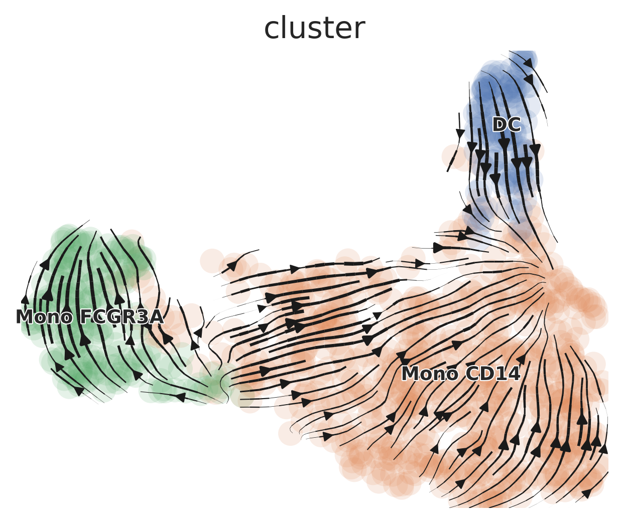

sessionInfo()

## R version 4.4.0 (2024-04-24)
## Platform: x86_64-pc-linux-gnu
## Running under: Ubuntu 20.04.6 LTS
## 
## Matrix products: default
## BLAS:   /usr/lib/x86_64-linux-gnu/blas/libblas.so.3.9.0 
## LAPACK: /usr/lib/x86_64-linux-gnu/lapack/liblapack.so.3.9.0
## 
## locale:
##  [1] LC_CTYPE=en_US.UTF-8       LC_NUMERIC=C              
##  [3] LC_TIME=de_BE.UTF-8        LC_COLLATE=en_US.UTF-8    
##  [5] LC_MONETARY=de_BE.UTF-8    LC_MESSAGES=en_US.UTF-8   
##  [7] LC_PAPER=de_BE.UTF-8       LC_NAME=C                 
##  [9] LC_ADDRESS=C               LC_TELEPHONE=C            
## [11] LC_MEASUREMENT=de_BE.UTF-8 LC_IDENTIFICATION=C       
## 
## time zone: Europe/Brussels
## tzcode source: system (glibc)
## 
## attached base packages:
## [1] stats4    tools     stats     graphics  grDevices utils     datasets 
## [8] methods   base     
## 
## other attached packages:
##  [1] slingshot_2.12.0            TrajectoryUtils_1.12.0     
##  [3] SingleCellExperiment_1.26.0 SummarizedExperiment_1.34.0
##  [5] Biobase_2.64.0              GenomicRanges_1.56.1       
##  [7] GenomeInfoDb_1.40.1         IRanges_2.38.1             
##  [9] S4Vectors_0.42.1            BiocGenerics_0.50.0        
## [11] MatrixGenerics_1.16.0       matrixStats_1.3.0          
## [13] princurve_2.1.6             rlang_1.1.4                
## [15] scales_1.3.0                dplyr_1.1.4                
## [17] mgcv_1.9-1                  nlme_3.1-165               
## [19] reshape2_1.4.4              viridis_0.6.5              
## [21] viridisLite_0.4.2           cowplot_1.1.3              
## [23] RColorBrewer_1.1-3          ggplot2_3.5.1              
## [25] reticulate_1.38.0           glue_1.7.0                 
## [27] hdf5r_1.3.11                SeuratExtend_1.1.0         
## [29] SeuratExtendData_0.2.1      Seurat_5.1.0               
## [31] SeuratObject_5.0.2          sp_2.1-4                   
## 
## loaded via a namespace (and not attached):
##   [1] RcppAnnoy_0.0.22          splines_4.4.0            
##   [3] later_1.3.2               tibble_3.2.1             
##   [5] polyclip_1.10-6           fastDummies_1.7.3        
##   [7] lifecycle_1.0.4           globals_0.16.3           
##   [9] lattice_0.22-6            MASS_7.3-61              
##  [11] magrittr_2.0.3            plotly_4.10.4            
##  [13] sass_0.4.9                rmarkdown_2.29           
##  [15] jquerylib_0.1.4           yaml_2.3.9               
##  [17] rlist_0.4.6.2             httpuv_1.6.15            
##  [19] sctransform_0.4.1         spam_2.10-0              
##  [21] spatstat.sparse_3.1-0     pbapply_1.7-2            
##  [23] abind_1.4-5               zlibbioc_1.50.0          
##  [25] Rtsne_0.17                purrr_1.0.2              
##  [27] rappdirs_0.3.3            GenomeInfoDbData_1.2.12  
##  [29] ggrepel_0.9.5             irlba_2.3.5.1            
##  [31] listenv_0.9.1             spatstat.utils_3.0-5     
##  [33] goftest_1.2-3             RSpectra_0.16-1          
##  [35] spatstat.random_3.2-3     fitdistrplus_1.2-1       
##  [37] parallelly_1.37.1         DelayedMatrixStats_1.26.0
##  [39] pkgdown_2.0.7             leiden_0.4.3.1           
##  [41] codetools_0.2-20          DelayedArray_0.30.1      
##  [43] tidyselect_1.2.1          UCSC.utils_1.0.0         
##  [45] farver_2.1.2              spatstat.explore_3.2-7   
##  [47] jsonlite_1.8.8            progressr_0.14.0         
##  [49] ggridges_0.5.6            survival_3.7-0           
##  [51] systemfonts_1.1.0         ragg_1.3.2               
##  [53] ica_1.0-3                 Rcpp_1.0.13              
##  [55] gridExtra_2.3             SparseArray_1.4.8        
##  [57] xfun_0.45                 withr_3.0.0              
##  [59] fastmap_1.2.0             fansi_1.0.6              
##  [61] digest_0.6.36             R6_2.5.1                 
##  [63] mime_0.12                 textshaping_0.4.0        
##  [65] colorspace_2.1-0          scattermore_1.2          
##  [67] tensor_1.5                spatstat.data_3.1-2      
##  [69] utf8_1.2.4                tidyr_1.3.1              
##  [71] generics_0.1.3            data.table_1.15.4        
##  [73] httr_1.4.7                htmlwidgets_1.6.4        
##  [75] S4Arrays_1.4.1            uwot_0.2.2               
##  [77] pkgconfig_2.0.3           gtable_0.3.5             
##  [79] lmtest_0.9-40             XVector_0.44.0           
##  [81] htmltools_0.5.8.1         dotCall64_1.1-1          
##  [83] png_0.1-8                 knitr_1.48               
##  [85] rstudioapi_0.16.0         cachem_1.1.0             
##  [87] zoo_1.8-12                stringr_1.5.1            
##  [89] KernSmooth_2.23-24        parallel_4.4.0           
##  [91] miniUI_0.1.1.1            desc_1.4.3               
##  [93] pillar_1.9.0              grid_4.4.0               
##  [95] vctrs_0.6.5               RANN_2.6.1               
##  [97] promises_1.3.0            xtable_1.8-4             
##  [99] cluster_2.1.6             evaluate_0.24.0          
## [101] cli_3.6.3                 compiler_4.4.0           
## [103] crayon_1.5.3              future.apply_1.11.2      
## [105] labeling_0.4.3            plyr_1.8.9               
## [107] fs_1.6.4                  stringi_1.8.4            
## [109] deldir_2.0-4              munsell_0.5.1            
## [111] lazyeval_0.2.2            spatstat.geom_3.2-9      
## [113] Matrix_1.7-0              RcppHNSW_0.6.0           
## [115] patchwork_1.2.0           sparseMatrixStats_1.16.0 
## [117] bit64_4.0.5               future_1.33.2            
## [119] shiny_1.8.1.1             highr_0.11               
## [121] ROCR_1.0-11               igraph_2.0.3             
## [123] memoise_2.0.1             bslib_0.4.2              
## [125] bit_4.0.5

Yichao Hua

2024-11-28

Table of Contents

Analyzing Single-Cell Trajectories with scVelo

Downloading Example Data

Preparing Data for scVelo

Generating scVelo Plots

Palantir Tutorial for Trajectory and Pseudotime Analysis

Introduction

Downloading Example Data

Running Diffusion Map

UMAP Based on “ms”

(Optional) Incorporating Newly Calculated Dimension Reductions into AnnData

Determining Cell Fates and Calculating Pseudotime

MAGIC for Denoising and Smoothing Gene Expression

CellRank Tutorial for Trajectory Analysis

Introduction

Adding Pseudotime to the adata Object

Running CellRank Kernel

Generating the Plots

Gene Expression Dynamics Along Differentiation Trajectories]

Gene Trend Curves with Palantir

Customizing Gene Trend Curves

Gene Trend Heatmaps with Palantir

Slingshot Tutorial for Pseudotime Analysis

Running Slingshot

Accessing Slingshot Output

Gene Trend Curves for Slingshot Pseudotime

Visualizing Gene Trends with Heatmaps

Integration of Seurat with Python Tools

Introduction

Creating a Conda Environment with All Required Python Packages

Integrating Seurat with AnnData

Converting Seurat Object to Loom

Importing Loom File into AnnData

Viewing AnnData Object

Adding Dimension Reduction Data

Direct Conversion from Seurat to AnnData

Updating AnnData with New Metadata

Saving and Loading AnnData

Adding Pseudotime to the `adata` Object