Lesson 5: Core scRNA-seq Workflow Enhancements

Introduction

In Lesson 2, we explored the basic workflow of single-cell analysis using a small PBMC dataset. While this served as an excellent introduction to the field, it only scratched the surface of what’s possible with single-cell RNA sequencing (scRNA-seq) analysis. In this lesson, we’ll delve deeper into various aspects of the workflow, exploring more advanced techniques and considerations.

We’ll cover the following topics:

Merging multiple datasets
Detailed quality control (nGene, percent.mt)
Doublet removal
Data integration
Cell-Cycle Scoring and Regression
Alternative normalization methods (SCTransform)

1. Merging Multiple Datasets

In real-world scenarios, we often need to analyze multiple datasets together. This could be due to various reasons, such as comparing different conditions, time points, or even different technologies used on the same sample.

For this exercise, we’ll use public datasets from the 10X Genomics website. These datasets are from the same sample but were processed using different technologies: the 3’ kit and the 5’ kit. These two approaches capture genes differently, which can lead to some variation in the results.

First, let’s set your working directory to where we’ll store all course materials. If you followed Lesson 1, this would be:

# Set working directory to the course folder created in Lesson 1
# If you used a different location, replace this path with your chosen directory
setwd("~/Documents/single-cell-course")

Load the necessary libraries and read in our data:

library(Seurat)
library(SeuratExtend)

# Load 3' dataset
pbmc_3p <- Read10X("data/pbmc_ACDA/3p_ACDA/filtered_feature_bc_matrix/")
pbmc_3p <- CreateSeuratObject(pbmc_3p, project = "pbmc_3p", min.features = 200, min.cells = 1)

# Load 5' dataset
pbmc_5p <- Read10X("data/pbmc_ACDA/5p_ACDA/filtered_feature_bc_matrix/")
pbmc_5p <- CreateSeuratObject(pbmc_5p, project = "pbmc_5p", min.features = 200, min.cells = 1)

# Merge the datasets
pbmc_merge <- merge(pbmc_3p, pbmc_5p, add.cell.ids = c("pbmc_3p","pbmc_5p"))
pbmc_merge <- JoinLayers(pbmc_merge) # This step is required for Seurat v5
pbmc_merge

## An object of class Seurat 
## 27910 features across 8845 samples within 1 assay 
## Active assay: RNA (27910 features, 0 variable features)
##  1 layer present: counts

By merging these datasets, we can compare and analyze them together. The add.cell.ids parameter adds a prefix to cell names to distinguish their origin after merging.

2. Detailed Quality Control (nGene, percent.mt)

In our previous lesson, we used a basic quality control criterion: min.features = 200, which retains cells with more than 200 detected genes. However, this is quite a low threshold, chosen because the previous dataset had a low sequencing depth. In practice, these thresholds need to be adjusted based on the specific characteristics of your data.

Let’s start by examining the distribution of detected genes (nGene) in our merged dataset:

VlnPlot2(pbmc_merge, features = "nFeature_RNA", group.by = "orig.ident")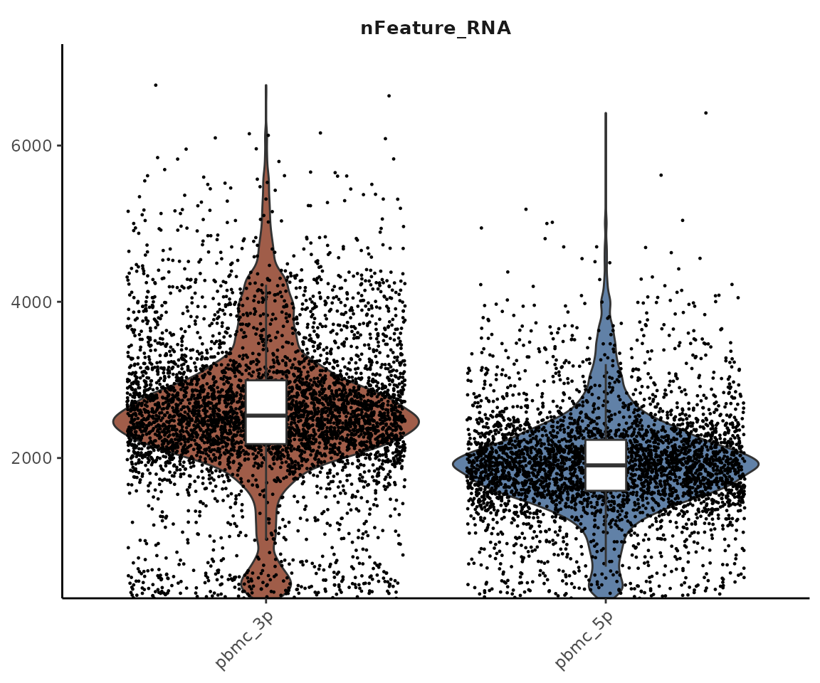

We can observe that the 3’ and 5’ technologies detect different numbers of genes. This difference is due to the nature of these technologies:

3’ Technology: This approach sequences the 3’ end of mRNA transcripts. It typically detects more genes and is more efficient, but it cannot perform TCR/BCR sequencing.
5’ Technology: This method sequences from the 5’ end of mRNA transcripts. It allows for TCR/BCR sequencing, making it particularly useful when studying different lymphocyte clones.

Setting nGene Thresholds

Cells with very low nGene are considered low quality and should be removed. The exact threshold depends on various factors including the sample type, cell type, and sequencing technology. Here are some general suggestions:

For 3’ sequencing: Usually set above 1000
For 5’ sequencing: Slightly lower, around 800-1000
For single nuclei sequencing: Even lower, typically 500-800

However, these are just general references. It’s crucial to examine the distribution in your data (using plots like the one above) to make an informed decision. For our current dataset, we’ll use 1000 as the lower threshold.

We also need to set an upper limit for nGene. While a higher nGene generally indicates better sequencing quality, extremely high values often represent anomalies such as doublets (two cells captured and sequenced as one). A common upper threshold is between 7500 and 8000 genes.

Note that this upper limit may need adjustment for certain technologies (e.g., Smart-seq2) that typically have higher sequencing depth, or for cell types (like fibroblasts or certain tumor cells) that naturally express more genes.

Mitochondrial Gene Percentage (percent.mt)

Another important quality control metric is the percentage of mitochondrial genes (percent.mt). A high percentage of mitochondrial reads often indicates low-quality or dying cells. This is because as cells die, their cytoplasmic mRNA degrades, but mitochondrial RNA is more stable, leading to a higher proportion of mitochondrial reads.

Let’s calculate and visualize the percent.mt for our dataset:

pbmc_merge[["percent.mt"]] <- PercentageFeatureSet(pbmc_merge, pattern = "^MT-")
VlnPlot2(pbmc_merge, features = "percent.mt", group.by = "orig.ident")

In this code, "^MT-" indicates genes starting with “MT-” (for human data). For mouse data, you would use "^mt-".

Typically, we set a threshold of percent.mt < 20%. For single nuclei data, which shouldn’t contain mitochondria, a stricter threshold like percent.mt < 5% is often used.

Applying Quality Control Filters

Now that we’ve discussed our quality control metrics, let’s apply these filters to our data:

# Before filtering
print(paste("Before filtering:", ncol(pbmc_merge), "cells"))

## [1] "Before filtering: 8845 cells"

# Apply filters
pbmc_merge <- subset(
  pbmc_merge,
  subset = nFeature_RNA > 1000 &
    nFeature_RNA < 7500 &
    percent.mt < 20
)

# After filtering
print(paste("After filtering:", ncol(pbmc_merge), "cells"))

## [1] "After filtering: 8256 cells"

By applying these filters, we’ve removed low-quality cells and potential doublets from our dataset, providing a cleaner foundation for downstream analysis.

3. Doublet Removal

In our previous section, we used a simple upper limit on nGene to remove potential doublets. However, this method is relatively crude. More sophisticated algorithms have been developed to identify and remove doublets with greater precision. One such tool is scDblFinder.

scDblFinder is a machine learning-based tool that identifies doublets in single-cell RNA sequencing data. It works by simulating artificial doublets from the existing data and then using these simulations to train a model that can distinguish real cells from doublets based on their gene expression profiles.

Before we begin, let’s ensure we have the necessary packages installed:

if (!require("BiocManager", quietly = TRUE))
  install.packages("BiocManager")
if (!require("scDblFinder", quietly = TRUE))
  BiocManager::install("scDblFinder")

Here’s how we can use scDblFinder in our analysis:

library(scDblFinder)

# Convert Seurat object to SingleCellExperiment
sce <- as.SingleCellExperiment(pbmc_merge)

# Run scDblFinder
sce <- scDblFinder(sce, samples = "orig.ident")

# Add scDblFinder results to our Seurat object
pbmc_merge$scDblFinder.class <- sce$scDblFinder.class

# View doublet predictions
table(pbmc_merge$scDblFinder.class)

## 
## singlet doublet 
##    7908     348

# Remove predicted doublets
pbmc_merge <- subset(pbmc_merge, subset = scDblFinder.class == "singlet")

# Check the number of cells after doublet removal
print(paste("After doublet removal:", ncol(pbmc_merge), "cells"))

## [1] "After doublet removal: 7908 cells"

For most standard single-cell RNA-seq analyses, using scDblFinder for doublet removal is a recommended practice that will improve your data quality. However, it’s important to keep in mind that like any computational method, it’s not 100% accurate. There are a few considerations to keep in mind:

False positives: Some cell types might be mistakenly identified as doublets. For example:
- Proliferating cells, which naturally have higher RNA content
- Rare cell types (like plasmacytoid dendritic cells, or pDCs) that may have unique gene expression profiles
Biological relevance: In some cases, what appears computationally as a “doublet” might be a biologically relevant state, such as cell-cell interactions or cells undergoing cell fusion.
Dataset specificity: The accuracy of doublet detection can vary depending on the characteristics of your dataset, including the cell types present and the sequencing technology used.

If you’re particularly interested in cell types that might be at risk of being misclassified as doublets, it’s advisable to carefully review the results before removing cells. You might consider:

Checking which cell types are disproportionately classified as doublets
Comparing the gene expression profiles of cells classified as doublets vs. singlets

Remember, the goal of doublet removal is to improve data quality, but it shouldn’t come at the cost of losing biologically relevant information. Always interpret the results in the context of your biological question and experimental design.

4. Data Integration

Now that we’ve performed quality control and doublet removal, let’s proceed with the traditional Seurat workflow on our merged PBMC dataset:

pbmc_merge <- NormalizeData(pbmc_merge)
pbmc_merge <- FindVariableFeatures(pbmc_merge)
pbmc_merge <- ScaleData(pbmc_merge)
pbmc_merge <- RunPCA(pbmc_merge)
pbmc_merge <- RunUMAP(pbmc_merge, dims = 1:10)
pbmc_merge <- FindNeighbors(pbmc_merge, dims = 1:10)
pbmc_merge <- FindClusters(pbmc_merge, resolution = 0.5)

## Modularity Optimizer version 1.3.0 by Ludo Waltman and Nees Jan van Eck
## 
## Number of nodes: 7908
## Number of edges: 272296
## 
## Running Louvain algorithm...
## Maximum modularity in 10 random starts: 0.9334
## Number of communities: 17
## Elapsed time: 0 seconds

DimPlot2(pbmc_merge, features = c("seurat_clusters", "orig.ident", "CD3D", "CD14"), theme = NoAxes())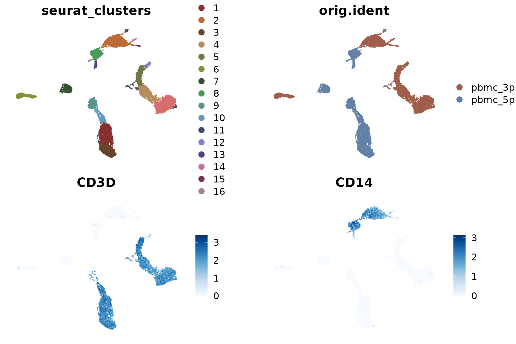

Upon examining the results, we notice that the clustering is significantly influenced by the different techniques used (3’ vs 5’ sequencing). This effect is known as batch effect. Ideally, we want our clustering to reflect the genuine cell type differences across all samples, rather than technical differences between batches.

To address this issue, we can use a method called Harmony for batch effect removal (or data integration). Harmony is an algorithm that adjusts for batch effects in single-cell data while preserving biological variation.

The principle behind Harmony is relatively straightforward: After running PCA, some principal components (PCs) reflect differences between cell clusters, while others represent differences between samples or batches. Harmony corrects for this by removing the PCs associated with batch differences while retaining those that represent genuine biological variation between cell types. This way, when we subsequently run UMAP and find clusters, the results will be based primarily on cell type differences rather than batch effects.

Let’s see how to implement Harmony:

First, if you haven’t installed Harmony, you can do so with the following code:

if (!require("harmony", quietly = TRUE))
    install.packages("harmony")

Now, let’s run Harmony (note that all steps up to and including RunPCA remain the same as before):

library(harmony)

## Loading required package: Rcpp

pbmc_merge <- RunHarmony(pbmc_merge, group.by.vars = "orig.ident")

## Transposing data matrix

## Initializing state using k-means centroids initialization

## Harmony 1/10

## Harmony 2/10

## Harmony 3/10

## Harmony 4/10

## Harmony 5/10

## Harmony converged after 5 iterations

After running Harmony, we proceed with the usual workflow, but now using the Harmony-corrected dimensions:

pbmc_merge <- RunUMAP(pbmc_merge, dims = 1:10, reduction = "harmony")
pbmc_merge <- FindNeighbors(pbmc_merge, dims = 1:10, reduction = "harmony")
pbmc_merge <- FindClusters(pbmc_merge, resolution = 0.5)

## Modularity Optimizer version 1.3.0 by Ludo Waltman and Nees Jan van Eck
## 
## Number of nodes: 7908
## Number of edges: 276741
## 
## Running Louvain algorithm...
## Maximum modularity in 10 random starts: 0.8982
## Number of communities: 12
## Elapsed time: 0 seconds

DimPlot2(pbmc_merge, features = c("seurat_clusters", "orig.ident", "CD3D", "CD14"), theme = NoAxes())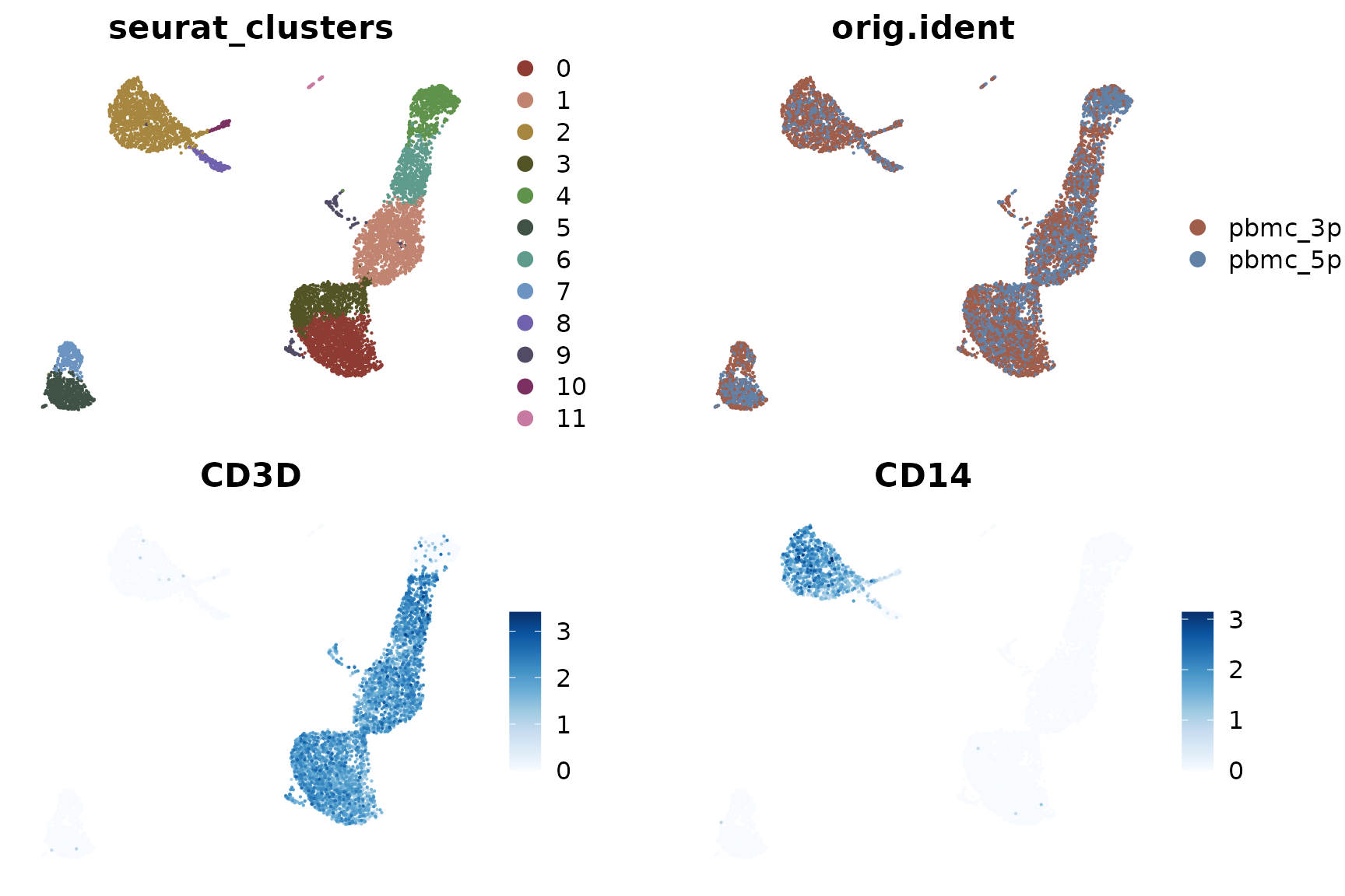

Now we can see that the clustering is based on cell types, and the differences between the two samples (3’ and 5’ sequencing) have been largely eliminated.

To better understand what Harmony has done, let’s compare the outputs of PCA and Harmony:

head(Embeddings(pbmc_merge, reduction = "pca"), 3)

##                                PC_1       PC_2      PC_3       PC_4       PC_5
## pbmc_3p_AAACCCAAGTGGTGGT-1 8.026468 -0.5569947 -9.762277  2.5274767  0.8005453
## pbmc_3p_AAACGAACACGTCGTG-1 5.573758  2.1691034 -5.162184 -0.4959971  0.2222917
## pbmc_3p_AAACGAAGTACCGGCT-1 8.495268 -0.5732680 -7.473360  2.3103625 -0.1895022
##                                  PC_6      PC_7       PC_8      PC_9      PC_10
## pbmc_3p_AAACCCAAGTGGTGGT-1 -2.0585799  3.759818 -3.4910666 1.7315773 -0.7347548
## pbmc_3p_AAACGAACACGTCGTG-1  0.4529012 -1.762161  2.7161359 0.5657139  0.7199774
## pbmc_3p_AAACGAAGTACCGGCT-1 -1.6952750  2.065426 -0.5903696 1.7199383  0.3588536
##                                 PC_11     PC_12      PC_13      PC_14
## pbmc_3p_AAACCCAAGTGGTGGT-1 -1.0875434 0.1700239  0.4207566 0.03125937
## pbmc_3p_AAACGAACACGTCGTG-1 -0.3842285 2.3215834 -2.2742613 0.82687791
## pbmc_3p_AAACGAAGTACCGGCT-1 -1.5259350 2.1005151 -0.8343805 1.95330595
##                                 PC_15      PC_16       PC_17    PC_18
## pbmc_3p_AAACCCAAGTGGTGGT-1 -0.5672855 -0.4333132  0.08478484 2.323176
## pbmc_3p_AAACGAACACGTCGTG-1 -0.9649320 -2.1877979 -0.12708595 1.235451
## pbmc_3p_AAACGAAGTACCGGCT-1 -0.4316831  0.1932790  0.25442805 1.317927
##                                 PC_19       PC_20      PC_21     PC_22
## pbmc_3p_AAACCCAAGTGGTGGT-1 -0.6686046  0.03036024 -0.0941112 0.1672879
## pbmc_3p_AAACGAACACGTCGTG-1 -0.8574119  0.03821086  1.2165595 0.8631614
## pbmc_3p_AAACGAAGTACCGGCT-1 -0.9668927 -1.37593441 -0.7858357 0.2565052
##                                 PC_23      PC_24      PC_25      PC_26
## pbmc_3p_AAACCCAAGTGGTGGT-1 -0.9431425 -1.0961104  1.5384187 -2.2628330
## pbmc_3p_AAACGAACACGTCGTG-1  0.4129460  0.4193254  0.3886109  0.7913914
## pbmc_3p_AAACGAAGTACCGGCT-1 -1.1181363 -0.4406358 -0.4530322  0.3490909
##                                 PC_27      PC_28      PC_29      PC_30
## pbmc_3p_AAACCCAAGTGGTGGT-1 -0.5962907 -1.2608390 -0.3187917  0.9369346
## pbmc_3p_AAACGAACACGTCGTG-1  0.2735535  0.4259994 -0.2572480 -0.8599530
## pbmc_3p_AAACGAAGTACCGGCT-1 -0.2951472 -0.5082128 -0.4150948  0.9005109
##                                PC_31      PC_32      PC_33      PC_34
## pbmc_3p_AAACCCAAGTGGTGGT-1 1.2749214  3.4092358  0.8348811 -0.0346970
## pbmc_3p_AAACGAACACGTCGTG-1 0.1665506 -0.8067949 -0.1263073 -0.5833165
## pbmc_3p_AAACGAAGTACCGGCT-1 1.3315582  0.3988518  0.2921252 -0.9007669
##                                 PC_35     PC_36      PC_37       PC_38
## pbmc_3p_AAACCCAAGTGGTGGT-1  2.5667212 2.3171880  0.5490577 -1.13369946
## pbmc_3p_AAACGAACACGTCGTG-1  2.3531437 0.8391040  1.0686152 -1.89676424
## pbmc_3p_AAACGAAGTACCGGCT-1 -0.8700297 0.4757511 -0.3616716  0.01687375
##                                 PC_39        PC_40      PC_41      PC_42
## pbmc_3p_AAACCCAAGTGGTGGT-1 -0.2095914  0.480441908 -2.7389293  0.2525975
## pbmc_3p_AAACGAACACGTCGTG-1  0.7896557 -2.035066291 -0.3943168 -0.5208215
## pbmc_3p_AAACGAAGTACCGGCT-1  0.9659524 -0.001937676  1.4530170  1.0012862
##                                PC_43       PC_44     PC_45      PC_46
## pbmc_3p_AAACCCAAGTGGTGGT-1 0.1412820 -1.73131972 -2.527521 -1.4119483
## pbmc_3p_AAACGAACACGTCGTG-1 0.5976390  0.38622614 -0.149614  1.5306139
## pbmc_3p_AAACGAAGTACCGGCT-1 0.3023768  0.08900624 -1.403962  0.0547492
##                                  PC_47      PC_48      PC_49       PC_50
## pbmc_3p_AAACCCAAGTGGTGGT-1 -0.01225440 -0.2481923 -0.6904021 -0.07385215
## pbmc_3p_AAACGAACACGTCGTG-1 -1.68094773  0.6444774 -0.4056492  0.37459072
## pbmc_3p_AAACGAAGTACCGGCT-1  0.04912378  1.5050713 -1.5763721  0.47545033

head(Embeddings(pbmc_merge, reduction = "harmony"), 3)

##                            harmony_1 harmony_2  harmony_3 harmony_4   harmony_5
## pbmc_3p_AAACCCAAGTGGTGGT-1  8.388242  1.335736 -4.8668592  4.084444  0.41571811
## pbmc_3p_AAACGAACACGTCGTG-1  6.167808  4.105549 -0.2162408  1.838270 -0.04784189
## pbmc_3p_AAACGAAGTACCGGCT-1  8.820353  1.359890 -2.4252238  3.893617 -0.54624121
##                             harmony_6  harmony_7  harmony_8  harmony_9
## pbmc_3p_AAACCCAAGTGGTGGT-1 -1.4299355  2.1941987 -3.4002057  0.4277696
## pbmc_3p_AAACGAACACGTCGTG-1  0.4370867 -2.3376343  1.5153617 -0.4987599
## pbmc_3p_AAACGAAGTACCGGCT-1 -1.0283993  0.5093963 -0.5792729  0.3888035
##                            harmony_10 harmony_11 harmony_12 harmony_13
## pbmc_3p_AAACCCAAGTGGTGGT-1 -0.9714052 -0.7872133 -0.2519855  0.3722271
## pbmc_3p_AAACGAACACGTCGTG-1  0.7019349 -0.3863685  1.3163239 -2.0239064
## pbmc_3p_AAACGAAGTACCGGCT-1  0.1175696 -1.2006624  1.5922227 -0.7882126
##                            harmony_14 harmony_15 harmony_16 harmony_17
## pbmc_3p_AAACCCAAGTGGTGGT-1 -0.2408347 -0.7151454  0.3595161  0.2865837
## pbmc_3p_AAACGAACACGTCGTG-1  0.2982565 -0.7589811 -1.2856362  0.3511975
## pbmc_3p_AAACGAAGTACCGGCT-1  1.6059979 -0.5914752  1.0340767  0.4834976
##                            harmony_18 harmony_19  harmony_20 harmony_21
## pbmc_3p_AAACCCAAGTGGTGGT-1   2.636532 -0.4950449  0.32679250  0.3099240
## pbmc_3p_AAACGAACACGTCGTG-1   1.543012 -0.5290196  0.02989942  1.3705860
## pbmc_3p_AAACGAAGTACCGGCT-1   1.599963 -0.7014958 -1.07391170 -0.3530896
##                            harmony_22 harmony_23  harmony_24 harmony_25
## pbmc_3p_AAACCCAAGTGGTGGT-1  0.2147109 -0.6313436 -1.00809759  1.3825846
## pbmc_3p_AAACGAACACGTCGTG-1  0.6656945  0.2965954  0.09918623  0.4108313
## pbmc_3p_AAACGAAGTACCGGCT-1  0.2676497 -0.8437084 -0.43827684 -0.5232299
##                            harmony_26 harmony_27  harmony_28  harmony_29
## pbmc_3p_AAACCCAAGTGGTGGT-1 -1.8557766 -0.5722115 -0.98298000 -0.16484030
## pbmc_3p_AAACGAACACGTCGTG-1  0.6545480  0.2271289 -0.08663837 -0.03217491
## pbmc_3p_AAACGAAGTACCGGCT-1  0.6936615 -0.3396854 -0.31663298 -0.30187817
##                            harmony_30 harmony_31 harmony_32 harmony_33
## pbmc_3p_AAACCCAAGTGGTGGT-1  1.0043036  1.1697774  2.9939500  0.9802589
## pbmc_3p_AAACGAACACGTCGTG-1 -0.7063055  0.4585552 -0.5126894 -0.3914611
## pbmc_3p_AAACGAAGTACCGGCT-1  0.8235596  1.2546143  0.1458695  0.4756327
##                             harmony_34 harmony_35 harmony_36 harmony_37
## pbmc_3p_AAACCCAAGTGGTGGT-1  0.06597315  2.4718136  2.3226729  0.5578287
## pbmc_3p_AAACGAACACGTCGTG-1 -0.52521668  2.1049645  0.8880769  1.0138088
## pbmc_3p_AAACGAAGTACCGGCT-1 -0.83771104 -0.8171414  0.4976160 -0.4034560
##                             harmony_38 harmony_39  harmony_40 harmony_41
## pbmc_3p_AAACCCAAGTGGTGGT-1 -1.19440293 -0.4690139  0.42072567 -2.7500936
## pbmc_3p_AAACGAACACGTCGTG-1 -1.78737338  0.9218403 -1.98124213 -0.3375522
## pbmc_3p_AAACGAAGTACCGGCT-1  0.05253346  0.6830896 -0.01472767  1.4352334
##                            harmony_42 harmony_43 harmony_44  harmony_45
## pbmc_3p_AAACCCAAGTGGTGGT-1  0.1544133  0.1317209 -1.6108667 -2.55868404
## pbmc_3p_AAACGAACACGTCGTG-1 -0.4857095  0.4854964  0.3541641 -0.03231285
## pbmc_3p_AAACGAAGTACCGGCT-1  0.9027680  0.2622781  0.1967017 -1.48418850
##                             harmony_46  harmony_47 harmony_48 harmony_49
## pbmc_3p_AAACCCAAGTGGTGGT-1 -1.46082294 -0.10673104 -0.1552405 -0.7432192
## pbmc_3p_AAACGAACACGTCGTG-1  1.54188352 -1.64739830  0.6040680 -0.4226623
## pbmc_3p_AAACGAAGTACCGGCT-1 -0.01742599 -0.04189954  1.6258599 -1.6174858
##                             harmony_50
## pbmc_3p_AAACCCAAGTGGTGGT-1 -0.01808169
## pbmc_3p_AAACGAACACGTCGTG-1  0.24020904
## pbmc_3p_AAACGAAGTACCGGCT-1  0.51006150

You’ll notice that they have the same shape. This is because Harmony essentially corrects the original PC matrix. To visualize this correction more clearly, let’s use Violin Plots to compare the first few PCA and Harmony dimensions:

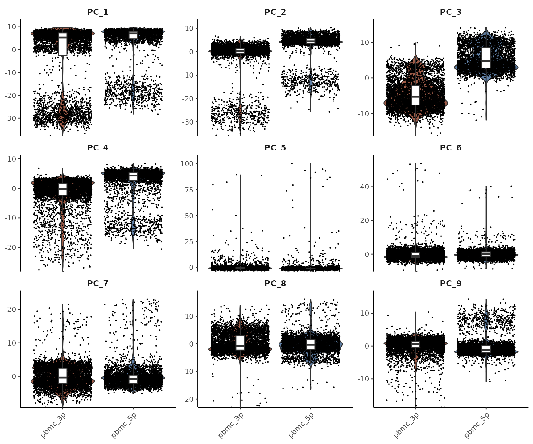
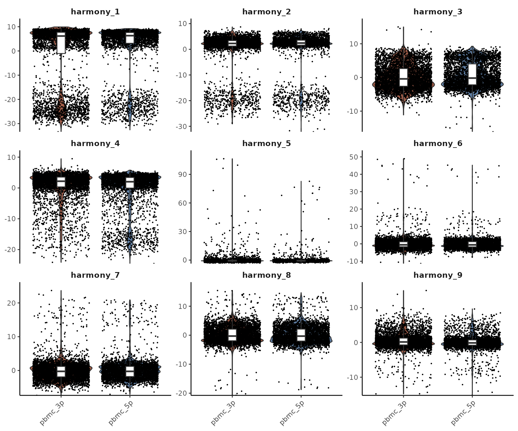
VlnPlot2(pbmc_merge, features = paste0("PC_", 1:9), group.by = "orig.ident")

VlnPlot2(pbmc_merge, features = paste0("harmony_", 1:9), group.by = "orig.ident")

As we can see, the PCs that were previously correlated with the orig.ident (i.e., showed clear differences between 3’ and 5’ samples) have been corrected. The Harmony-corrected PCs now primarily retain information about differences between cell types, rather than differences between sequencing techniques.

This integration step is crucial when working with multiple datasets or batches, as it allows us to focus on the biological differences of interest rather than technical variations between samples or batches. However, it’s important to use this technique judiciously and always consider whether the differences between your samples might be biologically relevant rather than just technical noise.

Let’s save the current Seurat object as an RDS file:

saveRDS(pbmc_merge, file = "rds/pbmc_merge.rds")

5. Cell-Cycle Scoring and Regression

When cells are in a state of division, they highly express cell cycle-related genes. These genes have such a strong signal that in unsupervised clustering, highly proliferating cells often form their own cluster, regardless of their original cell type. For example, in lymphocyte analysis, unsupervised clustering might identify various CD8, CD4 subgroups and NK cells, along with a cluster of mitotic cells. While this is often acceptable, there might be cases where you’re particularly interested in understanding which cell types these mitotic cells originally belonged to. In such situations, we need methods to mitigate the confounding effects of cell cycle genes.

This part of our tutorial is based on the Seurat vignette on cell cycle analysis: https://satijalab.org/seurat/articles/cell_cycle_vignette

Let’s start by calculating cell cycle scores:

# Load cell cycle genes
s.genes <- cc.genes$s.genes
g2m.genes <- cc.genes$g2m.genes

# Calculate cell cycle scores
pbmc_merge <- CellCycleScoring(pbmc_merge, s.features = s.genes, g2m.features = g2m.genes)

# View the results
head(pbmc_merge@meta.data)

##                            orig.ident nCount_RNA nFeature_RNA percent.mt
## pbmc_3p_AAACCCAAGTGGTGGT-1    pbmc_3p       6764         2301   7.140745
## pbmc_3p_AAACGAACACGTCGTG-1    pbmc_3p       5860         2212   6.621160
## pbmc_3p_AAACGAAGTACCGGCT-1    pbmc_3p       5616         2049   5.359687
## pbmc_3p_AAACGAATCGGAGTGA-1    pbmc_3p       6736         2879   8.283848
## pbmc_3p_AAACGCTAGATTGGGC-1    pbmc_3p       8285         2840   7.314424
## pbmc_3p_AAACGCTCAAAGCGTG-1    pbmc_3p       6333         2292   5.337123
##                            scDblFinder.class RNA_snn_res.0.5 seurat_clusters
## pbmc_3p_AAACCCAAGTGGTGGT-1           singlet               0               0
## pbmc_3p_AAACGAACACGTCGTG-1           singlet               1               1
## pbmc_3p_AAACGAAGTACCGGCT-1           singlet               3               3
## pbmc_3p_AAACGAATCGGAGTGA-1           singlet               2               2
## pbmc_3p_AAACGCTAGATTGGGC-1           singlet               0               0
## pbmc_3p_AAACGCTCAAAGCGTG-1           singlet               0               0
##                                 S.Score   G2M.Score Phase
## pbmc_3p_AAACCCAAGTGGTGGT-1  0.012127603  0.00916068     S
## pbmc_3p_AAACGAACACGTCGTG-1 -0.004794661  0.02908853   G2M
## pbmc_3p_AAACGAAGTACCGGCT-1  0.006306741  0.03890038   G2M
## pbmc_3p_AAACGAATCGGAGTGA-1 -0.059615105 -0.04554034    G1
## pbmc_3p_AAACGCTAGATTGGGC-1  0.034862991  0.03874900   G2M
## pbmc_3p_AAACGCTCAAAGCGTG-1 -0.007030940 -0.02781424    G1

After running CellCycleScoring, you’ll notice three new columns in the meta.data: - S.Score: The score for S phase - G2M.Score: The score for G2/M phase - Phase: The determined cell cycle phase for each cell

Once we’ve calculated these scores, we can regress out their effects during the data scaling step:

pbmc_merge <- ScaleData(pbmc_merge, vars.to.regress = c("S.Score", "G2M.Score"))

The rest of the workflow remains unchanged (i.e., you would proceed with RunPCA and subsequent steps as before).

Similarly, you can also regress out other confounding factors, such as the percentage of mitochondrial genes:

pbmc_merge <- ScaleData(pbmc_merge, vars.to.regress = c("S.Score", "G2M.Score", "percent.mt"))

It’s important to note that while we’re introducing this concept in class, we won’t be running these steps in our current analysis. The reason for introducing Cell-Cycle Regression is that some tutorials recommend doing this routinely. However, based on personal experience, this regression isn’t always effective, and whether to perform this step depends on your specific research goals.

Here are some considerations when deciding whether to perform cell cycle regression:

Research Question: If your research focuses on cell cycle-related processes or if you’re studying tissues with varying proliferation rates, you might want to retain this information rather than regress it out.
Biological Relevance: In some cases, the cell cycle state might be biologically relevant to your study. For instance, if you’re studying a developmental process or cancer, differences in proliferation rates between cell types or conditions could be important.
Effect on Other Genes: Regressing out cell cycle effects can sometimes impact the expression patterns of other genes, potentially obscuring other biological signals of interest.
Visualization: Sometimes, having a distinct cluster of mitotic cells can be informative and acceptable in your analysis, providing a quick visual cue about proliferating cells in your sample.
Downstream Analysis: Consider how cell cycle regression might affect any downstream analyses you plan to perform, such as trajectory inference or differential expression analysis.

In my personal opinion, retaining a cluster of mitotic cells in your cell clustering results is often acceptable and can be informative. However, the decision to regress out cell cycle effects should be made based on your specific research questions and the nature of your biological system.

If you do decide to perform cell cycle regression, it’s a good practice to compare your results before and after regression to understand how it’s affecting your data. This can help you make an informed decision about whether to include this step in your final analysis pipeline.

6. Alternative Normalization Methods (SCTransform)

So far, we’ve been using the NormalizeData function for data normalization. However, Seurat offers an alternative normalization method called SCTransform (for more details, see https://satijalab.org/seurat/articles/sctransform_vignette).

SCTransform is a powerful normalization method that aims to remove technical artifacts (e.g. Sequencing depth variations, Dropout events) from scRNA-seq data while preserving biological heterogeneity. It uses a regularized negative binomial regression model to normalize and transform the data, accounting for sequencing depth and other technical factors.

If you decide to use SCTransform, it replaces the combination of NormalizeData, FindVariableFeatures, and ScaleData steps in the traditional Seurat workflow. The rest of the workflow remains largely unchanged. Here’s an example of how to implement SCTransform:

if (!requireNamespace("glmGamPoi", quietly = TRUE)) 
    BiocManager::install("glmGamPoi")
options(future.globals.maxSize = 1000 * 1024^2)  # Increase to 1000 MiB

# Assuming pbmc_merge has been filtered for nGene and percent.mt, but not yet normalized

pbmc_merge <- SCTransform(pbmc_merge)
pbmc_merge <- RunPCA(pbmc_merge)
pbmc_merge <- RunHarmony(pbmc_merge, group.by.vars = "orig.ident", theta = 5) # Increase theta for stronger batch correction between 3' and 5' data
pbmc_merge <- RunUMAP(pbmc_merge, dims = 1:20, reduction = "harmony") # SCTransform often benefits from using more dimensions
pbmc_merge <- FindNeighbors(pbmc_merge, dims = 1:20, reduction = "harmony")
pbmc_merge <- FindClusters(pbmc_merge, resolution = 0.5)

## Modularity Optimizer version 1.3.0 by Ludo Waltman and Nees Jan van Eck
## 
## Number of nodes: 7908
## Number of edges: 279097
## 
## Running Louvain algorithm...
## Maximum modularity in 10 random starts: 0.9110
## Number of communities: 15
## Elapsed time: 0 seconds

DimPlot2(pbmc_merge, features = c("seurat_clusters", "orig.ident", "CD3D", "CD14"), theme = NoAxes())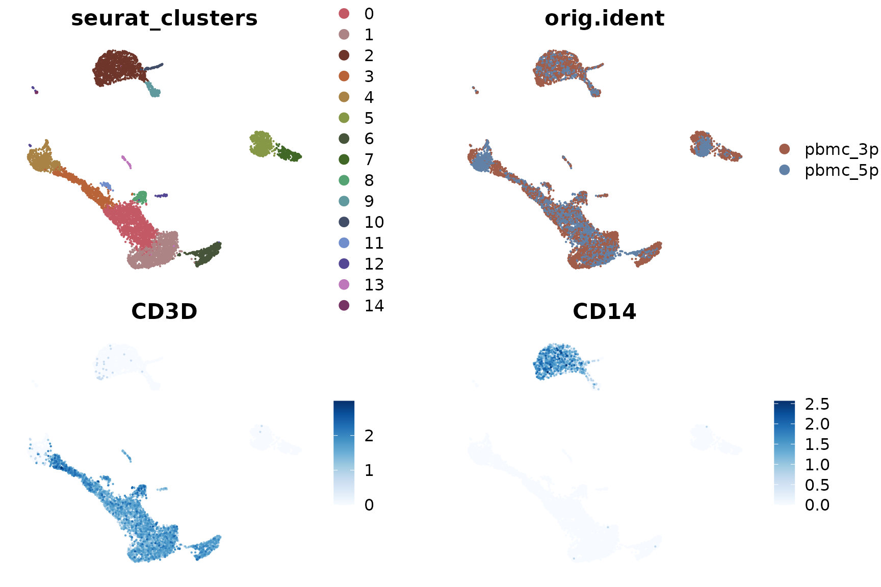

Both SCTransform and traditional normalization methods are widely accepted in the scRNA-seq analysis community. The authors of SCTransform argue that their method more effectively recovers true gene expression patterns and results in more refined clustering. However, there are some considerations to keep in mind:

Computational Resources: SCTransform typically requires more computational resources and storage space, especially for larger datasets.
Complex Microenvironments: For data from complex microenvironments (such as tumors), SCTransform may not always outperform traditional normalization methods.
Interpretability: The output of SCTransform can sometimes be less intuitive to interpret compared to traditional normalization methods.
Compatibility: Some downstream analysis tools might be optimized for traditionally normalized data, so it’s worth checking compatibility if you plan to use specialized analysis methods.

In my personal practice, I often run both methods and compare the results, choosing the one that provides clearer clustering, more distinct biological signatures, or better alignment with expected cell type distributions. This comparison can be particularly useful when working with a new dataset or biological system.

Here are some tips for comparing SCTransform with traditional normalization:

Visual Comparison: Compare UMAP plots from both methods. Look for clearer separation between cell types and more distinct clustering.
Marker Gene Expression: Check the expression patterns of known marker genes. The method that shows clearer and more biologically sensible patterns might be preferable.
Differential Expression Analysis: Perform differential expression analysis between clusters using both methods. Compare the results for biological relevance and consistency with prior knowledge.
Batch Effect Correction: If you’re working with multiple batches, compare how well each method handles batch effects.
Rare Cell Types: Pay attention to whether rare cell populations are better preserved or more clearly defined in one method versus the other.

Remember, the choice between SCTransform and traditional normalization should be based on your specific dataset, research questions, and computational resources. It’s always a good idea to critically evaluate the results and ensure they align with biological expectations and prior knowledge about your system.

7. Complete Workflow Summary

To conclude this lesson, let’s provide a comprehensive code block that encompasses all the steps we’ve covered. We’ll present two main workflows: one using the traditional NormalizeData approach, and another using SCTransform. Both workflows will include calculation of mitotic scores and regression of percent.mt, with an option to regress out mitotic scores if desired.

Traditional Workflow

# Load necessary libraries
library(Seurat)
library(SeuratExtend)
library(harmony)
library(scDblFinder)

# Load and merge datasets
pbmc_3p <- Read10X("data/pbmc_ACDA/3p_ACDA/filtered_feature_bc_matrix/")
pbmc_3p <- CreateSeuratObject(pbmc_3p, project = "pbmc_3p", min.features = 500, min.cells = 1)

pbmc_5p <- Read10X("data/pbmc_ACDA/5p_ACDA/filtered_feature_bc_matrix/")
pbmc_5p <- CreateSeuratObject(pbmc_5p, project = "pbmc_5p", min.features = 500, min.cells = 1)

pbmc_merge <- merge(pbmc_3p, pbmc_5p, add.cell.ids = c("pbmc_3p","pbmc_5p"))
pbmc_merge <- JoinLayers(pbmc_merge)

# Quality control
pbmc_merge[["percent.mt"]] <- PercentageFeatureSet(pbmc_merge, pattern = "^MT-")
pbmc_merge <- subset(
  pbmc_merge,
  subset = nFeature_RNA > 1000 &
    nFeature_RNA < 7500 &
    percent.mt < 20
)

# Doublet removal
sce <- as.SingleCellExperiment(pbmc_merge)
sce <- scDblFinder(sce, samples = "orig.ident")
pbmc_merge$scDblFinder.class <- sce$scDblFinder.class
pbmc_merge <- subset(pbmc_merge, subset = scDblFinder.class == "singlet")

# Traditional normalization and scaling
pbmc_merge <- NormalizeData(pbmc_merge)
pbmc_merge <- FindVariableFeatures(pbmc_merge)

# Calculate cell cycle scores
s.genes <- cc.genes$s.genes
g2m.genes <- cc.genes$g2m.genes
pbmc_merge <- CellCycleScoring(pbmc_merge, s.features = s.genes, g2m.features = g2m.genes)

# Scale data, regressing out percent.mt
# To regress out mitotic score, add "S.Score" and "G2M.Score" to vars.to.regress
pbmc_merge <- ScaleData(pbmc_merge, vars.to.regress = c("percent.mt"))

# Dimension reduction and clustering
pbmc_merge <- RunPCA(pbmc_merge)
pbmc_merge <- RunHarmony(pbmc_merge, group.by.vars = "orig.ident")
pbmc_merge <- RunUMAP(pbmc_merge, dims = 1:10, reduction = "harmony")
pbmc_merge <- FindNeighbors(pbmc_merge, dims = 1:10, reduction = "harmony")
pbmc_merge <- FindClusters(pbmc_merge, resolution = 0.5)

# Visualization
DimPlot2(pbmc_merge, features = c("seurat_clusters", "orig.ident", "CD3D", "CD14"), theme = NoAxes())

It’s worth mentioning that SeuratExtend provides a convenient function called RunBasicSeurat. This function integrates multiple steps including cell filtering, calculating percent.mt, as well as NormalizeData, FindVariableFeatures, ScaleData, RunPCA, RunHarmony, RunUMAP, FindNeighbors, and FindClusters into a single step, making it easier to use. Here’s an example of how to use it:

# Load necessary libraries
library(Seurat)
library(SeuratExtend)
library(scDblFinder)

# Load and merge datasets
pbmc_3p <- Read10X("data/pbmc_ACDA/3p_ACDA/filtered_feature_bc_matrix/")
pbmc_3p <- CreateSeuratObject(pbmc_3p, project = "pbmc_3p", min.features = 500, min.cells = 1)

pbmc_5p <- Read10X("data/pbmc_ACDA/5p_ACDA/filtered_feature_bc_matrix/")
pbmc_5p <- CreateSeuratObject(pbmc_5p, project = "pbmc_5p", min.features = 500, min.cells = 1)

pbmc_merge <- merge(pbmc_3p, pbmc_5p, add.cell.ids = c("pbmc_3p","pbmc_5p"))
pbmc_merge <- JoinLayers(pbmc_merge)

# Doublet removal
sce <- as.SingleCellExperiment(pbmc_merge)
sce <- scDblFinder(sce, samples = "orig.ident")
pbmc_merge$scDblFinder.class <- sce$scDblFinder.class
pbmc_merge <- subset(pbmc_merge, subset = scDblFinder.class == "singlet")

# Run the integrated workflow
pbmc_merge <- RunBasicSeurat(
  pbmc_merge,
  spe = "human",
  nFeature_RNA.min = 1000,
  nFeature_RNA.max = 7500,
  percent.mt.max = 20,
  dims = 1:10,
  resolution = 0.5,
  vars.to.regress = "percent.mt",
  harmony.by = "orig.ident"
)

# Visualization
DimPlot2(pbmc_merge, features = c("seurat_clusters", "orig.ident", "CD3D", "CD14"), theme = NoAxes())

This approach simplifies the workflow significantly, allowing you to perform multiple analysis steps with a single function call. It’s particularly useful for standard analyses or when you want to quickly process your data using default parameters.

SCTransform Workflow

# Load necessary libraries
library(Seurat)
library(SeuratExtend)
library(harmony)
library(scDblFinder)

# Load and merge datasets
pbmc_3p <- Read10X("data/pbmc_ACDA/3p_ACDA/filtered_feature_bc_matrix/")
pbmc_3p <- CreateSeuratObject(pbmc_3p, project = "pbmc_3p", min.features = 500, min.cells = 1)

pbmc_5p <- Read10X("data/pbmc_ACDA/5p_ACDA/filtered_feature_bc_matrix/")
pbmc_5p <- CreateSeuratObject(pbmc_5p, project = "pbmc_5p", min.features = 500, min.cells = 1)

pbmc_merge <- merge(pbmc_3p, pbmc_5p, add.cell.ids = c("pbmc_3p","pbmc_5p"))
pbmc_merge <- JoinLayers(pbmc_merge)

# Quality control
pbmc_merge[["percent.mt"]] <- PercentageFeatureSet(pbmc_merge, pattern = "^MT-")
pbmc_merge <- subset(
  pbmc_merge,
  subset = nFeature_RNA > 1000 &
    nFeature_RNA < 7500 &
    percent.mt < 20
)

# Doublet removal
sce <- as.SingleCellExperiment(pbmc_merge)
sce <- scDblFinder(sce, samples = "orig.ident")
pbmc_merge$scDblFinder.class <- sce$scDblFinder.class
pbmc_merge <- subset(pbmc_merge, subset = scDblFinder.class == "singlet")

# Calculate cell cycle scores
s.genes <- cc.genes$s.genes
g2m.genes <- cc.genes$g2m.genes
pbmc_merge <- CellCycleScoring(pbmc_merge, s.features = s.genes, g2m.features = g2m.genes)

# SCTransform normalization
# To regress out mitotic score, add "S.Score" and "G2M.Score" to vars.to.regress
pbmc_merge <- SCTransform(pbmc_merge, vars.to.regress = c("percent.mt"))

# Dimension reduction and clustering
pbmc_merge <- RunPCA(pbmc_merge)
pbmc_merge <- RunHarmony(pbmc_merge, group.by.vars = "orig.ident", theta = 5)
pbmc_merge <- RunUMAP(pbmc_merge, dims = 1:20, reduction = "harmony")
pbmc_merge <- FindNeighbors(pbmc_merge, dims = 1:20, reduction = "harmony")
pbmc_merge <- FindClusters(pbmc_merge, resolution = 0.5)

# Visualization
DimPlot2(pbmc_merge, features = c("seurat_clusters", "orig.ident", "CD3D", "CD14"), theme = NoAxes())

These comprehensive workflows incorporate all the key steps we’ve discussed in this lesson, including data loading, quality control, doublet removal, normalization (using both traditional and SCTransform methods), cell cycle scoring, batch correction with Harmony, and clustering.

Remember that the choice between the traditional workflow and SCTransform depends on your specific dataset and research questions. It’s often beneficial to try both methods and compare the results. Additionally, the decision to regress out mitotic scores should be based on your biological question and the nature of your data.

By providing these complete workflows, you can easily reproduce the entire analysis process and modify it as needed for your own datasets. Happy analyzing!

Yichao Hua

2024-11-29