What's New in v1.2.0 • SeuratExtend

New Features and Enhancements in v1.2.0

Dark Theme Support for Feature Plot Visualization

The FeaturePlot3 and FeaturePlot3.grid functions now support a dark theme option, providing better contrast for visualizing gene expression patterns, particularly in presentations or low-light environments:

library(Seurat)
library(SeuratExtend)

# Using dark theme with FeaturePlot3
FeaturePlot3(
  pbmc, 
  color = "rgb", 
  feature.1 = "CD3D", 
  feature.2 = "CD14", 
  feature.3 = "CD79A", 
  pt.size = 1,
  dark.theme = TRUE
)

New Violin Plot Styling Options

The VlnPlot2 function now supports an “outline” style option, which uses white-filled violins with colored outlines instead of the default filled style:

# Outline style for violin plots
genes <- c("CD3D", "CD14", "CD79A")
VlnPlot2(pbmc, features = genes, style = "outline", ncol = 1)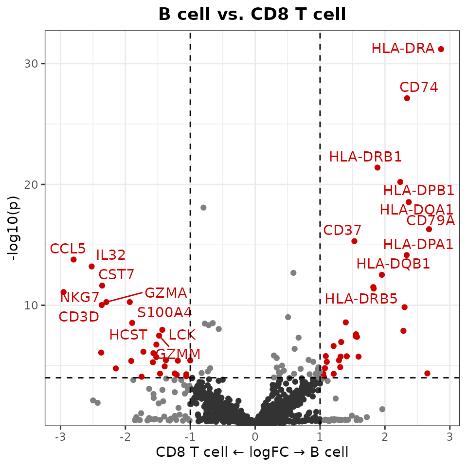

New ClusterDistrPlot Function

The new ClusterDistrPlot function extends ClusterDistrBar to allow comparison of cluster distribution patterns between experimental conditions. When the condition parameter is provided, it creates boxplots grouped by condition instead of stacked bars:

# Compare cluster distribution between conditions
ClusterDistrPlot(
  origin = pbmc$sample_id,
  cluster = pbmc$cluster,
  condition = pbmc$condition
)

This function inherits styling options from VlnPlot2 when in boxplot mode, making it highly versatile for comparing cell type proportions across experimental groups.

Enhanced Log Fold Change Options in Differential Analysis Plots

Both WaterfallPlot and VolcanoPlot functions now support different logarithm bases for fold change calculations through the log.base parameter:

# Using log base 2 for fold change calculations in WaterfallPlot
WaterfallPlot(
  pbmc, 
  group.by = "cluster", 
  features = VariableFeatures(pbmc)[1:80],
  ident.1 = "Mono CD14", 
  ident.2 = "CD8 T cell", 
  length = "logFC",
  log.base = "2",    # Use log2 instead of natural log
  top.n = 20)

# Using log base 2 in VolcanoPlot
VolcanoPlot(
  pbmc,
  ident.1 = "B cell",
  ident.2 = "CD8 T cell",
  log.base = "2"    # Use log2 instead of natural log
)

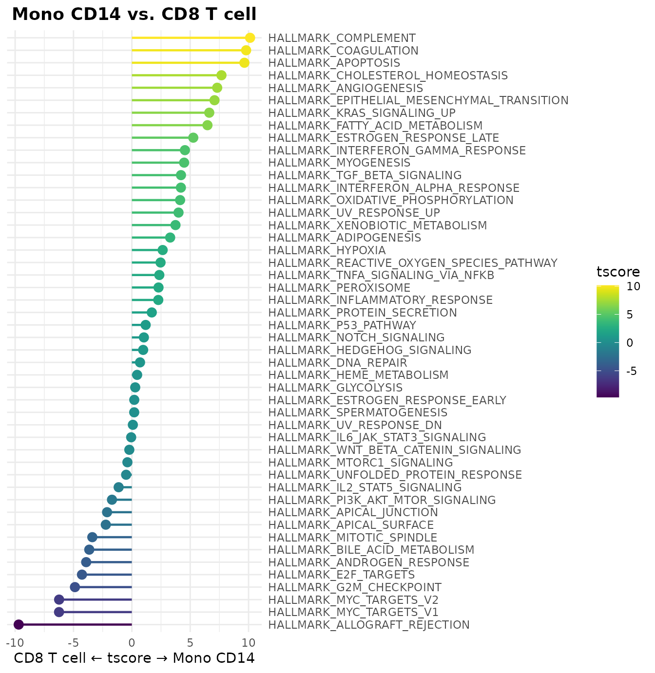
Available options include: - log.base = "e": Natural logarithm (default) - log.base = "2": Log base 2 - log.base = "10": Log base 10 - Any numeric value for custom bases

Color Scheme Updates

New “Bright” Color Scheme and Default Change

A new vibrant color scheme “bright” has been added for visualizations requiring higher contrast:

library(cowplot)
DimPlot2(pbmc, features = c("orig.ident", "cluster"), cols = "bright", ncol = 2, theme = NoAxes())

Based on user feedback, the default discrete color scheme has been changed from “default” (darker theme) to “light” to avoid color inconsistency in DimPlot2 when toggling between labeled and unlabeled displays.

If you prefer to retain the original “default” (darker) color scheme, you can use:

seu <- save_colors(seu, col_list = list("discrete" = "default"))

Enhanced Gene Set Enrichment Analysis (GSEA) Capabilities

Improved Database Management

SeuratExtend now offers enhanced ways to manage and update the GO and Reactome databases used in your GSEA analyses:

# Install specific versions of SeuratExtendData for different database releases
install_SeuratExtendData("latest")    # Latest version (April 2025 data)
install_SeuratExtendData("stable")    # Stable version (January 2020 data)
install_SeuratExtendData("v0.2.1")    # Specific version with January 2020 datasets
install_SeuratExtendData("v0.3.0")    # Specific version with April 2025 datasets

This ensures compatibility with specific analysis workflows or when you need to match results from previous studies.

Creating and Using Custom Databases

SeuratExtend now provides a more streamlined workflow for creating and using custom GO or Reactome databases:

# Load custom database
custom_GO_Data <- readRDS("path/to/your/GO_Data.rds")

# Use with SeuratExtend by assigning to global environment
GO_Data <- custom_GO_Data

# Run analysis
seu <- GeneSetAnalysisGO(seu, parent = "immune_system_process")

# When done, remove the global variable
rm(GO_Data)

This feature is particularly useful for: - Using the latest database updates - Creating databases for additional model organisms - Developing custom pathway collections

For detailed documentation on creating custom databases, SeuratExtend provides comprehensive guides accessible through:

browseURL("https://github.com/huayc09/SeuratExtendData/blob/main/inst/db_creation/README_GO_Data.md")
browseURL("https://github.com/huayc09/SeuratExtendData/blob/main/inst/db_creation/README_Reactome_Data.md")

Apple Silicon (M1/M2/M3/M4) Support for Trajectory Analysis

SeuratExtend v1.2.0 adds support for Apple Silicon chips (M1/M2/M3/M4), allowing macOS users to run Python-based trajectory analysis tools. However, this support comes with specific limitations that require following a particular workflow to avoid R session crashes:

# IMPORTANT: Apple Silicon users MUST initialize Python environment BEFORE loading any data
library(SeuratExtend)
activate_python()  # Must call this function FIRST to prevent memory-related crashes

# Only THEN load your data and proceed with analysis
seu <- readRDS("path/to/seurat_object.rds")

Important Considerations:

On Apple Silicon, memory management issues exist between R and Python, especially when performing operations like PCA on AnnData objects
If R objects are loaded before calling Python functions, the R session will likely crash
You must start a fresh R session and call activate_python() before loading any data
This initialization sequence is necessary when using tools like scVelo, Palantir, or CellRank

Despite these limitations, the create_condaenv_seuratextend() function now automatically detects Apple Silicon and uses the appropriate configuration, enabling Mac users to run:

scVelo: for RNA velocity analysis
Palantir: for cell fate determination and pseudotime analysis
CellRank: for trajectory analysis
MAGIC: for gene expression denoising and smoothing

Bug Fixes and Improvements

Several important bug fixes and enhancements have been implemented based on user feedback:

scVelo Functions: Fixed issues related to scVelo functionality, addressing reported bugs in GitHub issue #30.
DotPlot2: Fixed bugs affecting the appearance and functionality of the DotPlot2 function (GitHub issues #22 and #29).
Palantir Windows Compatibility: Fixed compatibility issues for Palantir functions on Windows systems (GitHub issue #24).
Color Palette Enhancement: Increased the color limit from 50 to 80 colors in the color_pro function, allowing for more color options in visualizations.
ClusterDistrBar Validation: Added input validation to the ClusterDistrBar function to prevent errors from invalid inputs.
RColorBrewer Sequential Palettes: Enhanced the lightest colors in sequential color palettes to improve visibility against white backgrounds.
VlnPlot2 Documentation: Added detailed explanations of the statistics options in the VlnPlot2 function documentation.
Package Installation: Fixed issues in the internal import function related to automatic package installation.
WaterfallPlot Improvements:
- Added automatic adjustment of x-axis text angle and alignment for better readability
- Added option to display borders around bars for improved visual clarity

New Features and Enhancements in v1.1.0

New Visualization Functions

Enhanced Dot Plots with `DotPlot2`

A new function DotPlot2 has been introduced, combining dot size (percent of expressing cells) with color intensity (average expression) for more informative visualizations:

library(Seurat)
library(SeuratExtend)

# With grouped features
grouped_features <- list(
  "B_cell_markers" = c("MS4A1", "CD79A"),
  "T_cell_markers" = c("CD3D", "CD8A", "IL7R"),
  "Myeloid_markers" = c("CD14", "FCGR3A", "S100A8")
)
DotPlot2(pbmc, features = grouped_features)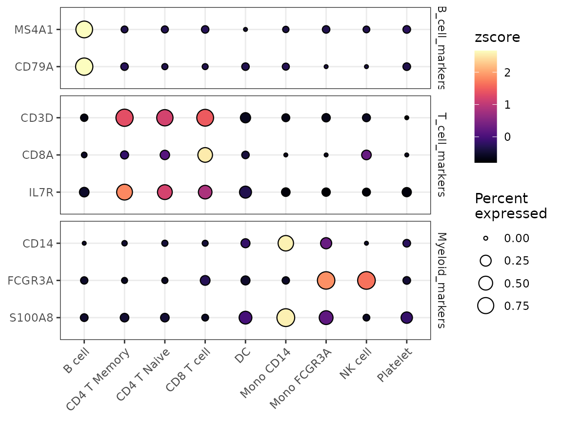

New Volcano Plots

The new VolcanoPlot function provides statistical visualization of differential expression:

VolcanoPlot(pbmc, 
            ident.1 = "B cell",
            ident.2 = "CD8 T cell")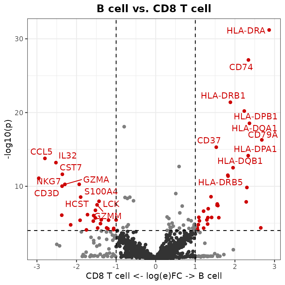

UMAP Arrow Annotations

Added theme_umap_arrows for simplified axis indicators on dimension reduction plots:

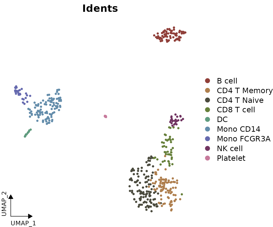
DimPlot2(pbmc, theme = NoAxes()) + theme_umap_arrows()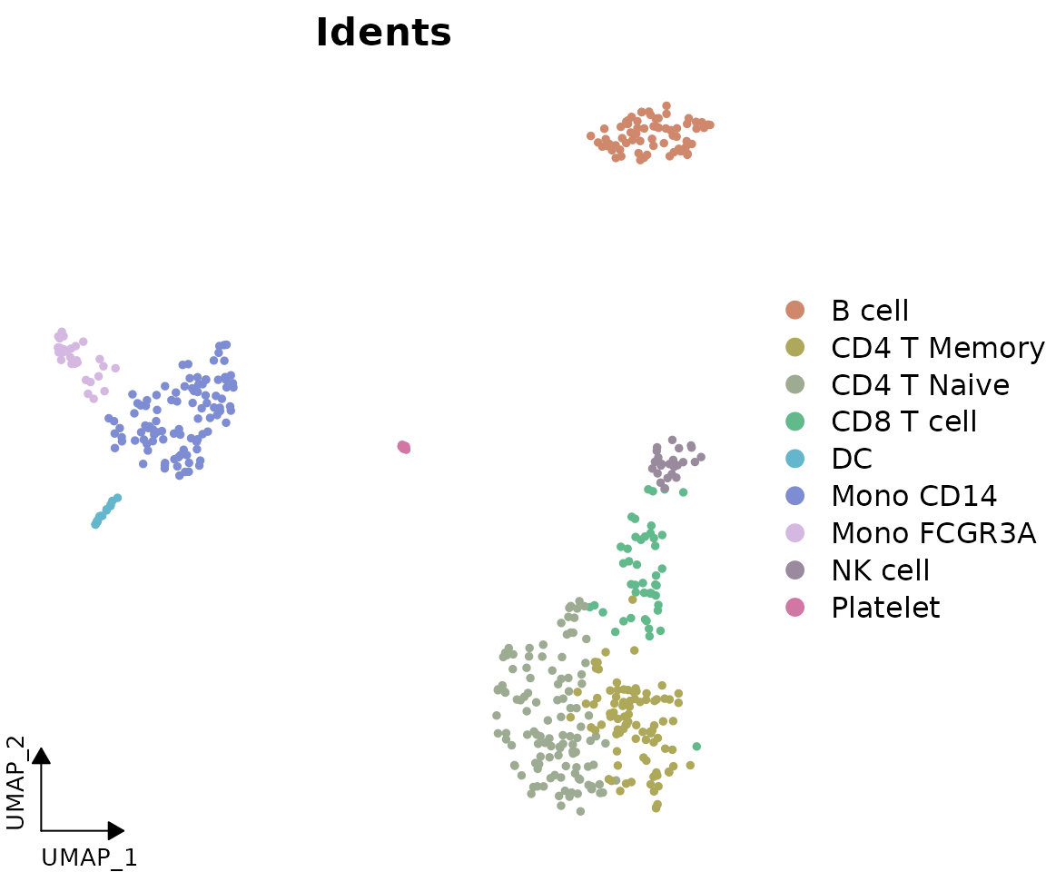

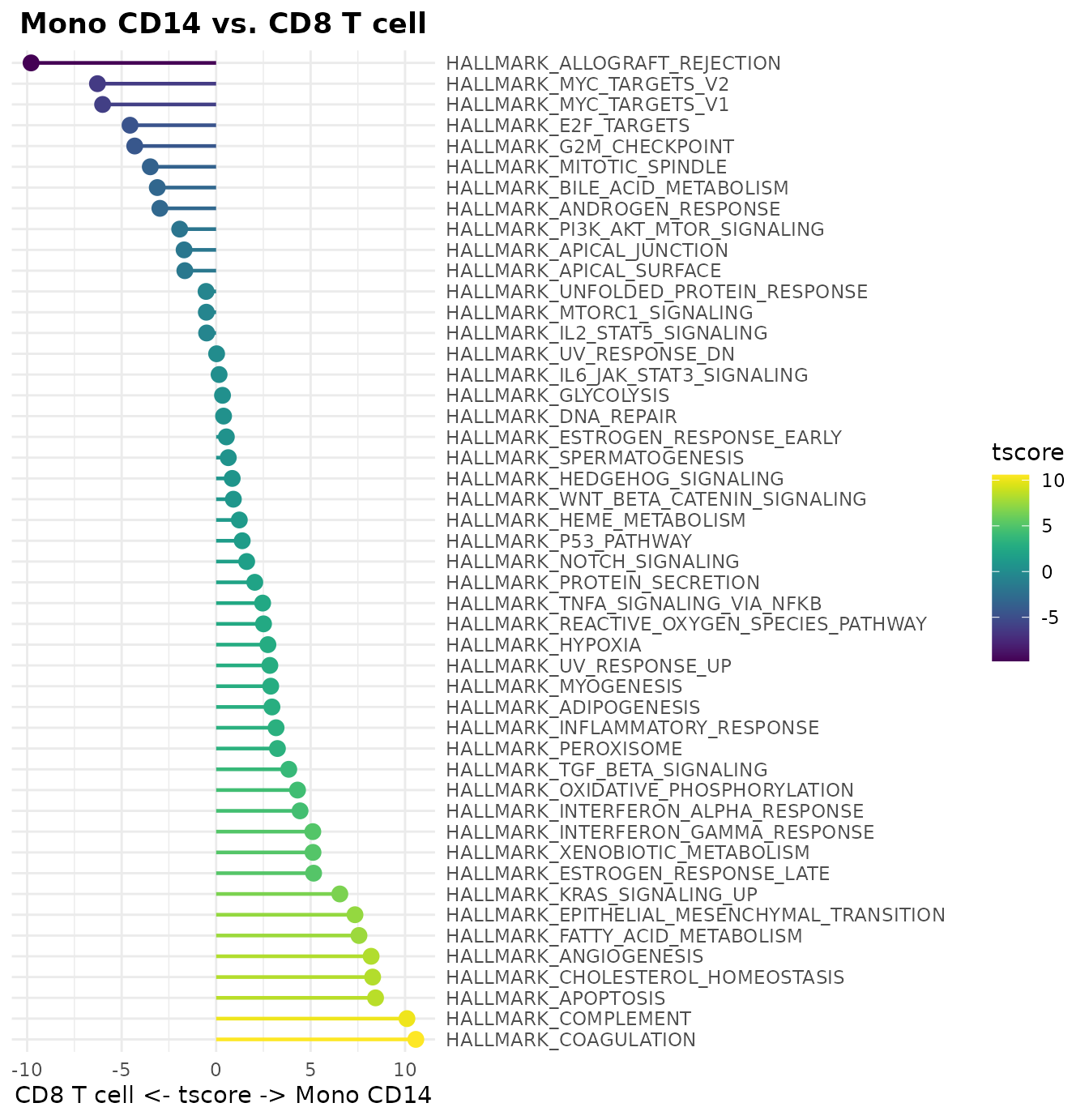
Enhanced Existing Functions

VlnPlot2 Enhancements

Added support for mean and median lines in violin plots:

VlnPlot2(pbmc, 
         features = c("CCR7", "IL7R", "TCF7"),
         cols = "light",
         show.mean = TRUE,      # Show mean and median lines
         mean_colors = c("red", "blue"),  # Colors for mean and median
         ncol = 1)

New WaterfallPlot Style: “segment”

Added a new visualization style “segment” to WaterfallPlot, providing an alternative way to display differences between conditions:

# Prepare data
pbmc <- GeneSetAnalysis(pbmc, genesets = hall50$human)
matr <- pbmc@misc$AUCell$genesets

# Create a plot using the new segment style
WaterfallPlot(
  matr,
  f = pbmc$cluster,
  ident.1 = "Mono CD14",
  ident.2 = "CD8 T cell",
  style = "segment",
  color_theme = "D"
)

Color Scheme Updates

New Default Color Schemes

Two major color scheme changes have been implemented in v1.1.0:

For continuous variables: Changed from viridis “A” to RColorBrewer “Blues”
For heatmaps: Updated from c(low = muted("blue"), mid = "white", high = muted("red")) to “BuRd”

Here are visual comparisons of the old and new defaults:

Continuous Variable Color Scheme

# Create a side-by-side comparison for continuous variables
library(cowplot)
library(ggpubr)

# Old default (viridis "A")
p1 <- DimPlot2(pbmc, 
               features = "CD3D", 
               cols = "A",  # Old default
               theme = theme_umap_arrows()) 

# New default (Blues)
p2 <- DimPlot2(pbmc, 
               features = "CD3D", 
               theme = theme_umap_arrows()) 

plot_grid(
  annotate_figure(p1, top = text_grob("Old Default (viridis 'A')", size = 14)), 
  annotate_figure(p2, top = text_grob("New Default ('Blues')", size = 14)),
  ncol = 2)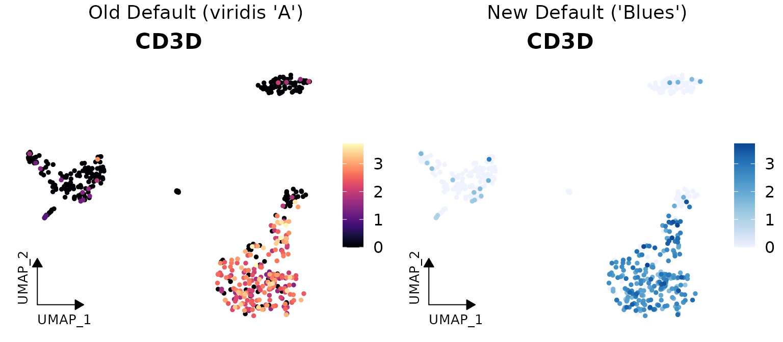

Heatmap Color Scheme

# Calculate data for heatmap
genes <- VariableFeatures(pbmc)
toplot <- CalcStats(pbmc, features = genes, method = "zscore", order = "p", n = 4)

# Create side-by-side heatmap comparison
p1 <- Heatmap(toplot, 
              color_scheme = c(low = scales::muted("blue"), 
                             mid = "white", 
                             high = scales::muted("red")), # Old default
              lab_fill = "zscore") +
      ggtitle("Old Default (blue-white-red)")

p2 <- Heatmap(toplot, 
              lab_fill = "zscore") +  # New default (BuRd) is automatically applied
      ggtitle("New Default ('BuRd')")

plot_grid(p1, p2, ncol = 2)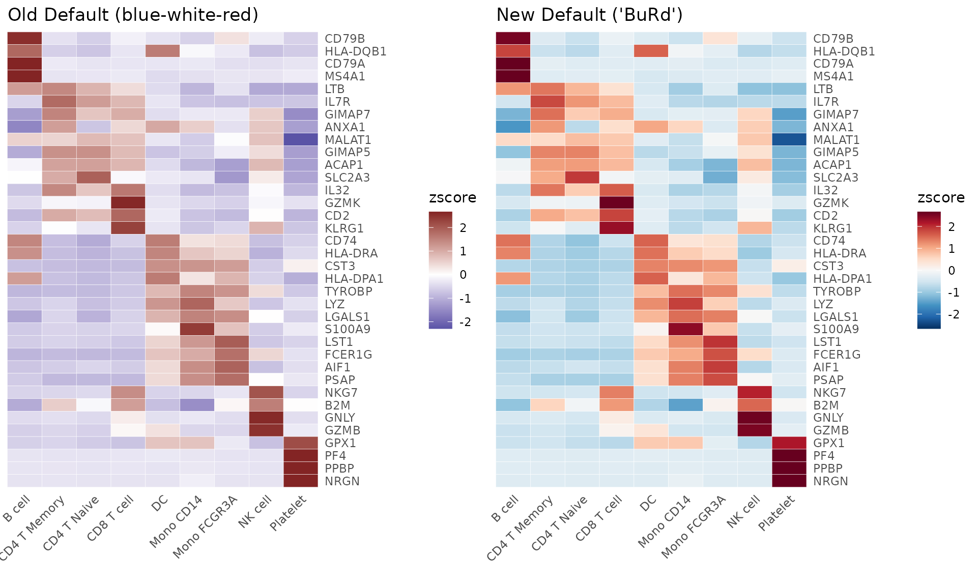

To revert to previous color schemes: - For continuous variables: Use cols = "A" - For heatmaps: Use color_scheme = c(low = scales::muted("blue"), mid = "white", high = scales::muted("red"))

New RColorBrewer Integration

Added support for RColorBrewer sequential and diverging palettes:

Sequential: “Blues”, “BuGn”, “BuPu”, “GnBu”, etc.
Diverging: “BrBG”, “PiYG”, “PRGn”, “PuOr”, etc.
Custom diverging: “GnYlRd”, “BuYlRd”, “GyRd”, “BuRd”, “PuOr”

Feature Enhancements

VlnPlot2: Now supports both stats.method and stat.method as parameter inputs (#10)
ClusterDistrBar: Added reverse_order parameter to adjust the stacking order (#11)
WaterfallPlot: Set upper limit for -log10(p) values to avoid NA issues (#14)
DimPlot2: Improved automatic point size adjustment and fixed point display issues in raster mode (#17)
show_col2: Function is now exported, allowing users to knit Visualization.Rmd without issues (#8)

Bug Fixes

VlnPlot2: Now explicitly uses dplyr::select internally to avoid conflicts with other packages’ select functions (#5, #10)
ClusterDistrBar: Fixed display issues when factor levels are numeric (e.g., seurat_clusters)

Documentation Updates

Conda Environment Setup

The create_condaenv_seuratextend() function documentation has been updated with important compatibility information:

Currently supported and tested on:
- Windows
- Intel-based macOS (not Apple Silicon/M1/M2)
- Linux (Ubuntu 20.04)

Note for Apple Silicon Users: The function is not currently compatible with Apple Silicon/M1/M2 devices (#7). Users with Apple Silicon devices who are interested in contributing to the development of M1/M2 support are welcome to reach out via GitHub Issues.

Windows-Specific File Download

When downloading loom files (which are HDF5-based binary files) on Windows, it’s essential to use mode = "wb" in the download.file() function:

# Example for Windows users
download.file("https://example.com/file.loom", "file.loom", mode = "wb")

This prevents Windows from modifying line endings in the binary file, which would corrupt the HDF5 format. Mac and Linux users don’t require this parameter, but including it is harmless.

sessionInfo()

## R version 4.4.0 (2024-04-24)
## Platform: x86_64-pc-linux-gnu
## Running under: Ubuntu 20.04.6 LTS
## 
## Matrix products: default
## BLAS:   /usr/lib/x86_64-linux-gnu/blas/libblas.so.3.9.0 
## LAPACK: /usr/lib/x86_64-linux-gnu/lapack/liblapack.so.3.9.0
## 
## locale:
##  [1] LC_CTYPE=en_US.UTF-8       LC_NUMERIC=C              
##  [3] LC_TIME=de_BE.UTF-8        LC_COLLATE=en_US.UTF-8    
##  [5] LC_MONETARY=de_BE.UTF-8    LC_MESSAGES=en_US.UTF-8   
##  [7] LC_PAPER=de_BE.UTF-8       LC_NAME=C                 
##  [9] LC_ADDRESS=C               LC_TELEPHONE=C            
## [11] LC_MEASUREMENT=de_BE.UTF-8 LC_IDENTIFICATION=C       
## 
## time zone: Europe/Brussels
## tzcode source: system (glibc)
## 
## attached base packages:
## [1] stats4    grid      stats     graphics  grDevices utils     datasets 
## [8] methods   base     
## 
## other attached packages:
##  [1] rlang_1.1.4               DelayedMatrixStats_1.26.0
##  [3] DelayedArray_0.30.1       SparseArray_1.4.8        
##  [5] S4Arrays_1.4.1            abind_1.4-5              
##  [7] IRanges_2.38.1            S4Vectors_0.42.1         
##  [9] MatrixGenerics_1.16.0     matrixStats_1.3.0        
## [11] BiocGenerics_0.50.0       mosaic_1.9.1             
## [13] mosaicData_0.20.4         ggformula_0.12.0         
## [15] Matrix_1.7-0              lattice_0.22-6           
## [17] cowplot_1.1.3             ggrepel_0.9.5            
## [19] viridis_0.6.5             viridisLite_0.4.2        
## [21] scales_1.3.0              tidyr_1.3.1              
## [23] ggbeeswarm_0.7.2          rlist_0.4.6.2            
## [25] RColorBrewer_1.1-3        dplyr_1.1.4              
## [27] ggpubr_0.6.0              ggplot2_3.5.1            
## [29] reshape2_1.4.4            SeuratExtend_1.2.0       
## [31] SeuratExtendData_0.3.0    Seurat_5.2.1             
## [33] SeuratObject_5.0.2        sp_2.1-4                 
## 
## loaded via a namespace (and not attached):
##   [1] RcppAnnoy_0.0.22         splines_4.4.0            later_1.3.2             
##   [4] tibble_3.2.1             polyclip_1.10-6          fastDummies_1.7.3       
##   [7] lifecycle_1.0.4          rstatix_0.7.2            globals_0.16.3          
##  [10] MASS_7.3-61              backports_1.5.0          magrittr_2.0.3          
##  [13] plotly_4.10.4            sass_0.4.9               rmarkdown_2.29          
##  [16] jquerylib_0.1.4          yaml_2.3.9               httpuv_1.6.15           
##  [19] sctransform_0.4.1        spam_2.10-0              spatstat.sparse_3.1-0   
##  [22] reticulate_1.38.0        pbapply_1.7-2            zlibbioc_1.50.0         
##  [25] Rtsne_0.17               purrr_1.0.2              labelled_2.13.0         
##  [28] irlba_2.3.5.1            listenv_0.9.1            spatstat.utils_3.0-5    
##  [31] goftest_1.2-3            RSpectra_0.16-1          spatstat.random_3.2-3   
##  [34] fitdistrplus_1.2-1       parallelly_1.37.1        pkgdown_2.0.7           
##  [37] codetools_0.2-20         tidyselect_1.2.1         farver_2.1.2            
##  [40] spatstat.explore_3.2-7   jsonlite_1.8.8           progressr_0.14.0        
##  [43] ggridges_0.5.6           survival_3.7-0           systemfonts_1.1.0       
##  [46] tools_4.4.0              ragg_1.3.2               ica_1.0-3               
##  [49] Rcpp_1.0.13              glue_1.7.0               gridExtra_2.3           
##  [52] xfun_0.45                withr_3.0.0              fastmap_1.2.0           
##  [55] fansi_1.0.6              digest_0.6.36            R6_2.5.1                
##  [58] mime_0.12                textshaping_0.4.0        colorspace_2.1-0        
##  [61] scattermore_1.2          tensor_1.5               spatstat.data_3.1-2     
##  [64] utf8_1.2.4               generics_0.1.3           data.table_1.15.4       
##  [67] httr_1.4.7               htmlwidgets_1.6.4        uwot_0.2.2              
##  [70] pkgconfig_2.0.3          gtable_0.3.5             lmtest_0.9-40           
##  [73] XVector_0.44.0           htmltools_0.5.8.1        carData_3.0-5           
##  [76] dotCall64_1.1-1          png_0.1-8                knitr_1.48              
##  [79] rstudioapi_0.16.0        nlme_3.1-165             cachem_1.1.0            
##  [82] zoo_1.8-12               stringr_1.5.1            KernSmooth_2.23-24      
##  [85] parallel_4.4.0           miniUI_0.1.1.1           vipor_0.4.7             
##  [88] desc_1.4.3               pillar_1.9.0             vctrs_0.6.5             
##  [91] RANN_2.6.1               promises_1.3.0           car_3.1-2               
##  [94] xtable_1.8-4             cluster_2.1.6            beeswarm_0.4.0          
##  [97] evaluate_0.24.0          cli_3.6.3                compiler_4.4.0          
## [100] crayon_1.5.3             future.apply_1.11.2      ggsignif_0.6.4          
## [103] labeling_0.4.3           plyr_1.8.9               forcats_1.0.0           
## [106] fs_1.6.4                 stringi_1.8.4            deldir_2.0-4            
## [109] munsell_0.5.1            lazyeval_0.2.2           spatstat.geom_3.2-9     
## [112] mosaicCore_0.9.4.0       RcppHNSW_0.6.0           hms_1.1.3               
## [115] patchwork_1.2.0          sparseMatrixStats_1.16.0 future_1.33.2           
## [118] shiny_1.8.1.1            highr_0.11               haven_2.5.4             
## [121] ROCR_1.0-11              igraph_2.0.3             broom_1.0.6             
## [124] memoise_2.0.1            bslib_0.4.2

What’s New in v1.2.0

Yichao Hua

2025-05-16

New Features and Enhancements in v1.2.0

Dark Theme Support for Feature Plot Visualization

New Violin Plot Styling Options

New ClusterDistrPlot Function

Enhanced Log Fold Change Options in Differential Analysis Plots

Color Scheme Updates

New “Bright” Color Scheme and Default Change

Enhanced Gene Set Enrichment Analysis (GSEA) Capabilities

Improved Database Management

Creating and Using Custom Databases

Apple Silicon (M1/M2/M3/M4) Support for Trajectory Analysis

Bug Fixes and Improvements

New Features and Enhancements in v1.1.0

New Visualization Functions

Enhanced Dot Plots with `DotPlot2`

New Volcano Plots

UMAP Arrow Annotations

Enhanced Existing Functions

VlnPlot2 Enhancements

New WaterfallPlot Style: “segment”

Color Scheme Updates

New Default Color Schemes

Continuous Variable Color Scheme

Heatmap Color Scheme

New RColorBrewer Integration

Feature Enhancements

Bug Fixes

Documentation Updates

Conda Environment Setup

Windows-Specific File Download

What’s New in v1.2.0

Yichao Hua

2025-05-16

New Features and Enhancements in v1.2.0

Dark Theme Support for Feature Plot Visualization

New Violin Plot Styling Options

New ClusterDistrPlot Function

Enhanced Log Fold Change Options in Differential Analysis Plots

Color Scheme Updates

New “Bright” Color Scheme and Default Change

Enhanced Gene Set Enrichment Analysis (GSEA) Capabilities

Improved Database Management

Creating and Using Custom Databases

Apple Silicon (M1/M2/M3/M4) Support for Trajectory Analysis

Bug Fixes and Improvements

New Features and Enhancements in v1.1.0

New Visualization Functions

Enhanced Dot Plots with DotPlot2

New Volcano Plots

UMAP Arrow Annotations

Enhanced Existing Functions

VlnPlot2 Enhancements

New WaterfallPlot Style: “segment”

Color Scheme Updates

New Default Color Schemes

Continuous Variable Color Scheme

Heatmap Color Scheme

New RColorBrewer Integration

Feature Enhancements

Bug Fixes

Documentation Updates

Conda Environment Setup

Windows-Specific File Download

Enhanced Dot Plots with `DotPlot2`