Lesson 2: Basic Single-Cell Analysis Workflow with Seurat

Introduction to Single-Cell Analysis with Seurat

Seurat is the most popular framework for analyzing single-cell data in R. It provides structured data storage, basic analysis workflows, and visualization solutions. Before we dive into the code, let’s introduce some fundamental concepts and principles of single-cell data analysis. This background will help us better understand the process.

From Raw Data to Visualization: The Single-Cell Analysis Journey

When we first receive sequencing data, it’s typically in the form of FASTQ files. These are text files that contain the raw nucleotide sequences. A typical FASTQ file looks like this:

FASTQ File Example

A key milestone in our single-cell analysis journey is to visualize cells using a UMAP (Uniform Manifold Approximation and Projection) plot, with colors distinguishing different cell clusters:

UMAP Example

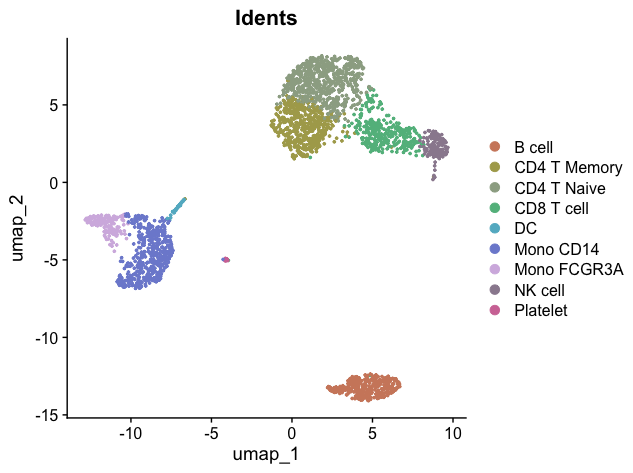
So, what happens between the raw FASTQ files and the final UMAP visualization? Here’s a simplified flowchart of the process:

Single-Cell Analysis Flowchart

Let’s break down each step of this process:

1. Mapping

This step aligns the raw sequences from the FASTQ files to a reference genome, resulting in a gene count matrix:

Gene Count Matrix

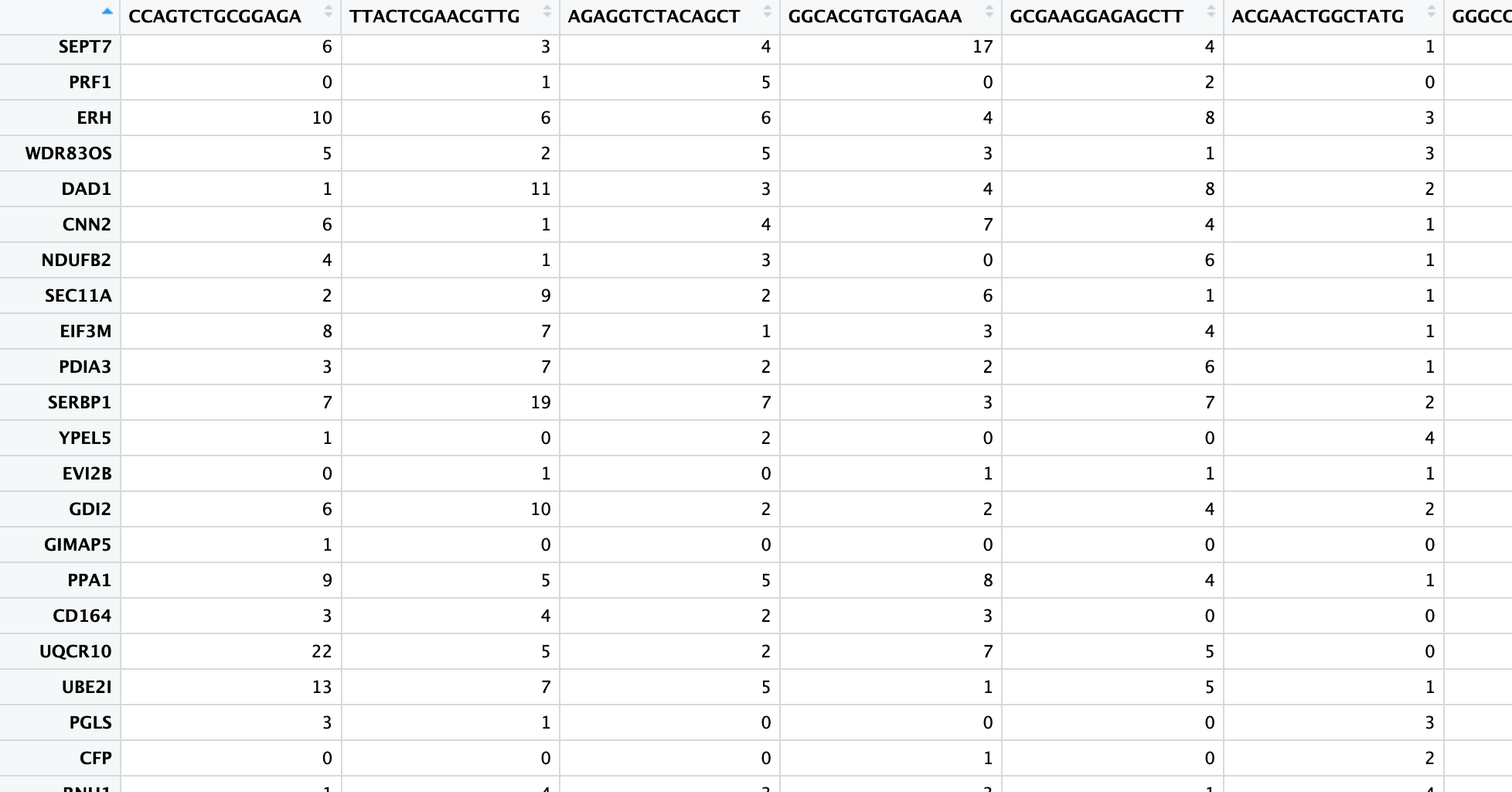
In this matrix: - Rows represent gene names - Columns represent cell names - Each cell contains a non-negative integer representing the number of reads for each gene in each cell

A “read” is an important concept - it represents one RNA fragment. For 10X sequencing data, this step is typically performed using CellRanger on a Linux server rather than a personal computer.

2. Data Normalization

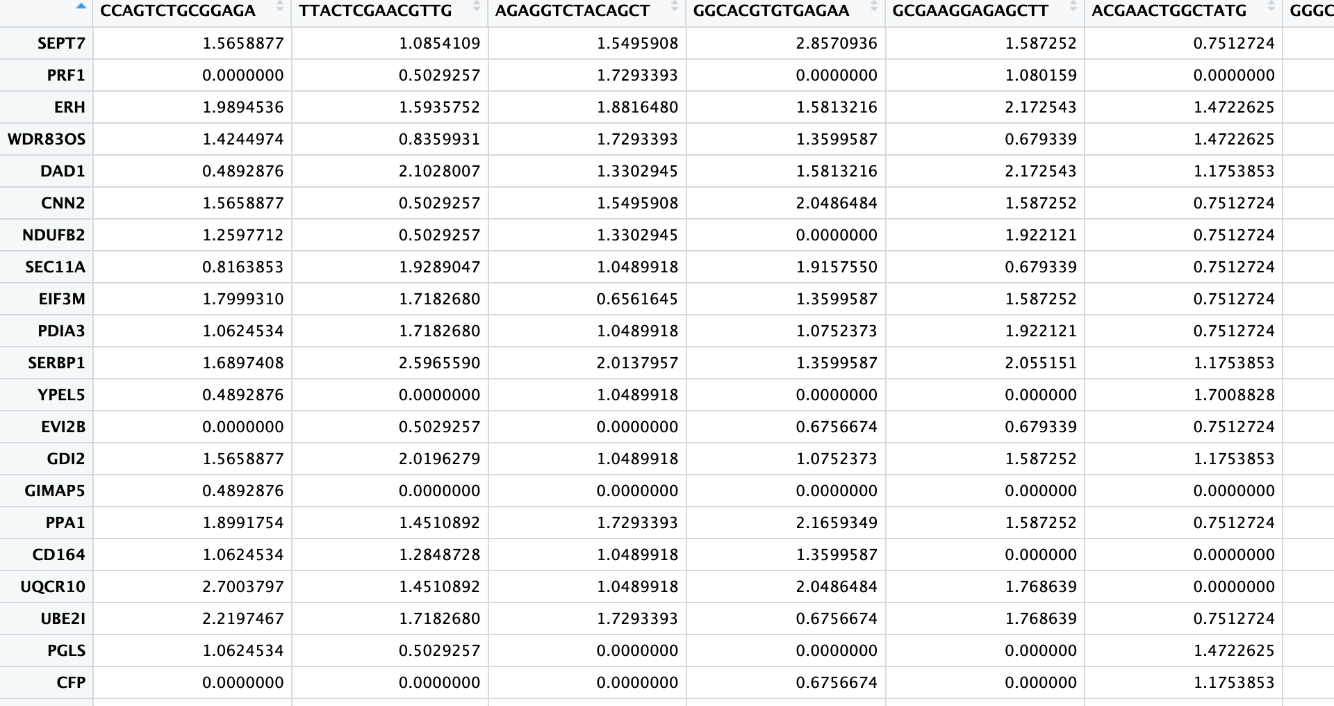
From this point onwards, we’ll be working on our personal computers. When we import the gene count matrix, we can’t use it directly for analysis because each cell has a different sequencing depth and read count, making direct comparisons impossible. Normalization addresses this issue in two steps:

Normalize by library size
Log transform

The result is a matrix of the same size as the gene count matrix, but containing normalized gene expression values:

Normalized Gene Expression

3. PCA (1st Dimension Reduction)

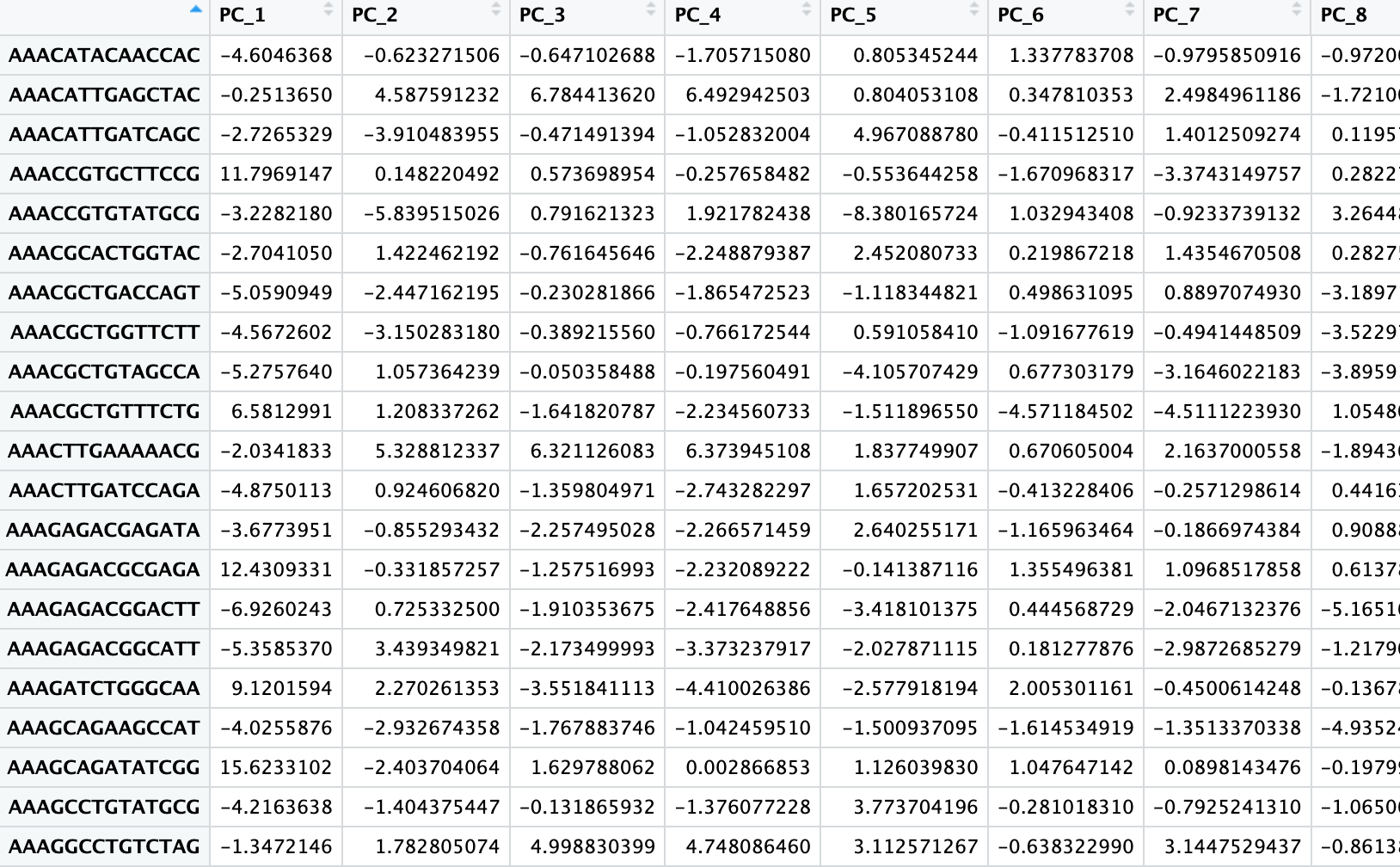
Principal Component Analysis (PCA) is our first step in dimension reduction. The original data has too many dimensions (e.g., 20,000 genes or features), making direct analysis computationally intensive. PCA reduces this to about 20-50 principal components (PCs).

We can roughly understand each PC as representing a group of genes that characterize or distinguish different cell types. For example, PC1 might relate to macrophages, PC2 to lymphocytes, and so on. Using PC1 and PC2, we can start to distinguish between macrophages, lymphocytes, and other cell types.

The output of this step is still a matrix, but much smaller than the original normalized matrix. It changes from a row (~20k genes) x column (cells) matrix to a row (cells) x column (20-50 PCs) matrix:

PCA Output

4. Unsupervised Clustering

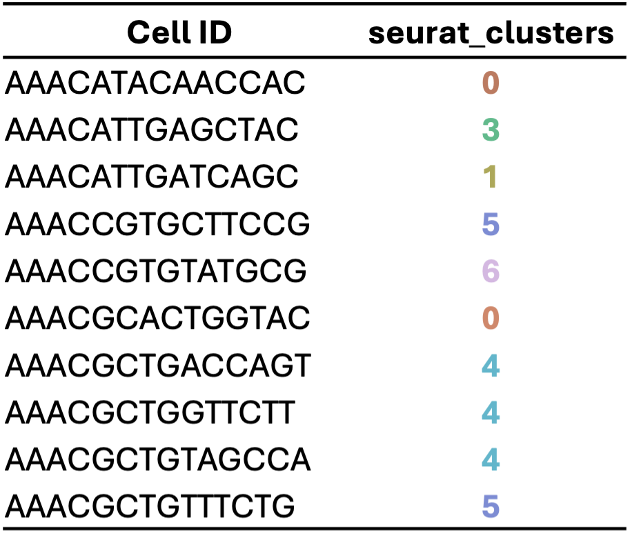
After the first PCA dimension reduction, we perform two parallel steps. One of these is unsupervised clustering.

Imagine a three-dimensional space where each point represents a cell. Cells that are closer in this space have more similar characteristics, so we group nearby cells into the same cluster. While our brains can only visualize three dimensions, computers can work in higher dimensions.

Using information from a selected number of top PCs (often ranging from 10 to 50, depending on the dataset), algorithms help us find and group similar cells in this high-dimensional space. The optimal number of PCs to use can vary based on the complexity and characteristics of your data.

Unsupervised Clustering

5. Visualization: UMAP/t-SNE (2nd Dimension Reduction)

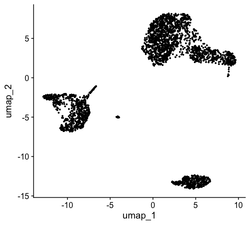
While the first PCA reduction allows us to distinguish some major groups using PC1 and PC2, more detailed grouping information might be contained in later PCs. To visualize this information in a two-dimensional plot, we need a second dimension reduction step. The most commonly used method for this is UMAP (Uniform Manifold Approximation and Projection).

UMAP compresses the multi-dimensional PC information (e.g. top 10-50 PCs, depending on the dataset) into two dimensions, allowing us to visualize cell differences more intuitively. The number of PCs used should be optimized for each dataset. This step gives us x-y coordinate points for each cell:

UMAP Coordinates

6. Final Visualization

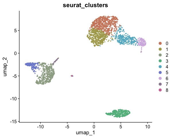
Finally, we combine the information from unsupervised clustering and UMAP. We plot each cell on the UMAP coordinates and color-code them based on their cluster assignment. This gives us the standard UMAP plot we aim for in single-cell analysis:

Final UMAP

This overview covers the basic workflow and principles of single-cell analysis. In the next section, we’ll learn how to implement these steps using R code and the Seurat package.

Implementing Single-Cell Analysis with Seurat

Now that we understand the basic workflow, let’s implement these steps using R code and the Seurat package.

1. Load Required Libraries

Before we begin, make sure you have installed the Seurat package. If you haven’t, you can install it using:

# install.packages("Seurat")

Now, let’s load the library:

library(Seurat)

2. Load the Data

First, let’s set your working directory to where we’ll store all course materials. If you followed Lesson 1, this would be:

# Set working directory to the course folder created in Lesson 1
# If you used a different location, replace this path with your chosen directory
setwd("~/Documents/single-cell-course")

Now let’s download and extract the course data:

# Download the course data (this may take a few minutes depending on your internet connection)
download.file(
  "https://zenodo.org/records/14245429/files/single-cell-course-data.zip",
  destfile = "course_data.zip"
)

# Extract the downloaded zip file
unzip("course_data.zip", exdir = "data")

We’ll be using a pre-downloaded 10x Genomics dataset of 3k PBMCs (Peripheral Blood Mononuclear Cells). The original dataset is available from this link. The data should now be in a folder named “data/pbmc3k/filtered_gene_bc_matrices/”.

This is a typical format for a gene count matrix from 10X CellRanger output. It includes three files: barcodes, genes/features, and matrix. We’ll use Seurat’s Read10X function to read this information into R:

raw_matrix <- Read10X("data/pbmc3k/filtered_gene_bc_matrices/")
raw_matrix[101:120,1:20]

## 20 x 20 sparse Matrix of class "dgCMatrix"

##   [[ suppressing 20 column names 'AAACATACAACCAC-1', 'AAACATTGAGCTAC-1', 'AAACATTGATCAGC-1' ... ]]

##                                                      
## GABRD         . . . . . . . . . . . . . . . . . . . .
## RP11-547D24.3 . . . . . . . . . . . . . . . . . . . .
## PRKCZ         . . . . . . . . . . . . . . . . . . . .
## RP5-892K4.1   . . . . . . . . . . . . . . . . . . . .
## RP11-181G12.2 . . . . . . . . . . . . . . . . . . . .
## C1orf86       . . . . . . . . 1 . . . . . . . . . . .
## AL590822.2    . . . . . . . . . . . . . . . . . . . .
## AL590822.1    . . . . . . . . . . . . . . . . . . . .
## RP11-181G12.5 . . . . . . . . . . . . . . . . . . . .
## RP11-181G12.4 . . . . . . . . . . . . . . . . . . . .
## SKI           . . . . . . . . . . . . . . . . . . . .
## MORN1         . . . . . . . . . . . . . . . . . . . .
## AL589739.1    . . . . . . . . . . . . . . . . . . . .
## RER1          . 1 1 1 . . . . . . . 1 . 1 . . . . 2 .
## PEX10         . . . . . . . . . . . . . . . . . . . .
## PLCH2         . . . . . . . . . . . . . . . . . . . .
## RP3-395M20.2  . . . . . . . . . . . . . . . . . . . .
## RP3-395M20.3  . . . . . . . . . . . . . . . . . . . .
## PANK4         . . 1 . . 1 . . . . . . . . . . . . . .
## HES5          . . . . . . . . . . . . . . . . . . . .

The code above extracts a portion of the raw count matrix. You’ll see that rows represent genes, columns represent cells, and the values are non-negative integers.

3. Create a Seurat Object

A Seurat object is one of the standardized formats for storing single-cell data. Let’s create one:

pbmc <- CreateSeuratObject(
  raw_matrix,
  min.features = 200,  # Keep cells with at least 200 detected genes
  project = "pbmc_3k", # Name of the project
  min.cells = 1        # Keep genes detected in at least 1 cell
)

## Warning: Feature names cannot have underscores ('_'), replacing with dashes
## ('-')

Let’s take a closer look at our Seurat object. The structure of a Seurat object is similar to a list, but with a key difference: Seurat objects have fixed slots, while list elements can be arbitrarily added or removed. We access slots in a Seurat object using the @ symbol.

To explore the object:

View(pbmc)  # Opens a viewer to explore the object

There’s a lot of information here, which we’ll gradually become familiar with. For now, let’s focus on two crucial components:

The raw count matrix:

pbmc@assays$RNA$counts[1:20, 1:20]  # View a small portion of the raw count matrix

## 20 x 20 sparse Matrix of class "dgCMatrix"

##   [[ suppressing 20 column names 'AAACATACAACCAC-1', 'AAACATTGAGCTAC-1', 'AAACATTGATCAGC-1' ... ]]

##                                                       
## AL627309.1    . . . . . . . . . . . . . . . . . . .  .
## AP006222.2    . . . . . . . . . . . . . . . . . . .  .
## RP11-206L10.2 . . . . . . . . . . . . . . . . . . .  .
## RP11-206L10.9 . . . . . . . . . . . . . . . . . . .  .
## FAM87B        . . . . . . . . . . . . . . . . . . .  .
## LINC00115     . . . . . . . . . . . . . . . . . . .  .
## FAM41C        . . . . . . . . . . . . . . . . . . .  .
## SAMD11        . . . . . . . . . . . . . . . . . . .  .
## NOC2L         . . . . . . . . . . . 1 . . . . . . .  .
## KLHL17        . . . . . . . . . . . . . . . . . . .  .
## PLEKHN1       . . . . . . . . . . . . . . . . . . .  .
## RP11-54O7.17  . . . . . . . . . . . . . . . . . . .  .
## HES4          . . . . . . . . . . . . . . . . . . 1  .
## RP11-54O7.11  . . . . . . . . . . . . . . . . . . .  .
## ISG15         . . 1 9 . 1 . . . 3 . . 1 5 . 2 1 1 1  .
## AGRN          . . . . . . . . . . . . . . . . . . .  .
## C1orf159      . . . . . . . . . . . . . . . . . . .  .
## TNFRSF18      . 2 . . . . . . . . . . . . . . . . .  .
## TNFRSF4       . . . . . . . . 1 . . . . . . . . . . 12
## SDF4          . . 1 . . . . . . . . . . . . . . . .  1

The meta.data, a data frame storing information about all cells:

head(pbmc@meta.data)  # View metadata associated with cells

##                  orig.ident nCount_RNA nFeature_RNA
## AAACATACAACCAC-1    pbmc_3k       2421          781
## AAACATTGAGCTAC-1    pbmc_3k       4903         1352
## AAACATTGATCAGC-1    pbmc_3k       3149         1131
## AAACCGTGCTTCCG-1    pbmc_3k       2639          960
## AAACCGTGTATGCG-1    pbmc_3k        981          522
## AAACGCACTGGTAC-1    pbmc_3k       2164          782

Seurat automatically creates three columns in the meta.data:

orig.ident: Usually indicates the sample source (we only have one sample here)
nFeature_RNA: Refers to nGene, the number of genes detected in the cell
nCount_RNA: Refers to the number of reads, representing sequencing depth

If we want to add cell-related information later (such as clustering or treatment conditions), we’ll add it to meta.data.

You can view all cell names and gene names using colnames() and rownames():

head(colnames(pbmc), 10)  # View cell names

##  [1] "AAACATACAACCAC-1" "AAACATTGAGCTAC-1" "AAACATTGATCAGC-1" "AAACCGTGCTTCCG-1"
##  [5] "AAACCGTGTATGCG-1" "AAACGCACTGGTAC-1" "AAACGCTGACCAGT-1" "AAACGCTGGTTCTT-1"
##  [9] "AAACGCTGTAGCCA-1" "AAACGCTGTTTCTG-1"

head(rownames(pbmc), 10)  # View gene names

##  [1] "AL627309.1"    "AP006222.2"    "RP11-206L10.2" "RP11-206L10.9"
##  [5] "FAM87B"        "LINC00115"     "FAM41C"        "SAMD11"       
##  [9] "NOC2L"         "KLHL17"

4. Normalize the Data

This step adjusts for differences in sequencing depth between cells:

pbmc <- NormalizeData(pbmc)

## Normalizing layer: counts

Let’s view a portion of the normalized data:

pbmc@assays$RNA$data[1:20, 1:10]

## 20 x 10 sparse Matrix of class "dgCMatrix"

##   [[ suppressing 10 column names 'AAACATACAACCAC-1', 'AAACATTGAGCTAC-1', 'AAACATTGATCAGC-1' ... ]]

##                                                                           
## AL627309.1    . .        .        .       . .        . . .        .       
## AP006222.2    . .        .        .       . .        . . .        .       
## RP11-206L10.2 . .        .        .       . .        . . .        .       
## RP11-206L10.9 . .        .        .       . .        . . .        .       
## FAM87B        . .        .        .       . .        . . .        .       
## LINC00115     . .        .        .       . .        . . .        .       
## FAM41C        . .        .        .       . .        . . .        .       
## SAMD11        . .        .        .       . .        . . .        .       
## NOC2L         . .        .        .       . .        . . .        .       
## KLHL17        . .        .        .       . .        . . .        .       
## PLEKHN1       . .        .        .       . .        . . .        .       
## RP11-54O7.17  . .        .        .       . .        . . .        .       
## HES4          . .        .        .       . .        . . .        .       
## RP11-54O7.11  . .        .        .       . .        . . .        .       
## ISG15         . .        1.429261 3.55831 . 1.726522 . . .        3.339271
## AGRN          . .        .        .       . .        . . .        .       
## C1orf159      . .        .        .       . .        . . .        .       
## TNFRSF18      . 1.625141 .        .       . .        . . .        .       
## TNFRSF4       . .        .        .       . .        . . 2.178946 .       
## SDF4          . .        1.429261 .       . .        . . .        .

5. Identify Variable Features

According to our previously discussed workflow, the next step would be the first dimension reduction using PCA. However, before running PCA, we need to perform two preparatory steps. The first is to find highly variable genes, typically defaulting to 2000 genes.

We don’t usually need all genes for cell clustering; we only need the genes with the most variation, as these often best reflect the differences between cell types.

pbmc <- FindVariableFeatures(pbmc)  # Identify genes that are highly variable across cells

## Finding variable features for layer counts

head(VariableFeatures(pbmc), 20)  # View the variable features

##  [1] "PPBP"     "LYZ"      "S100A9"   "IGLL5"    "GNLY"     "FTL"     
##  [7] "PF4"      "FTH1"     "GNG11"    "FCER1A"   "HLA-DRA"  "S100A8"  
## [13] "CD74"     "CLU"      "GZMB"     "NKG7"     "C1QA"     "CST3"    
## [19] "CCL4"     "HLA-DPB1"

6. Scale the Data and Perform PCA (Principal Component Analysis)

After finding variable genes, we need to convert their absolute expression values (non-negative numbers) into relative expression values centered around 0 (Scale data). We won’t delve into the mathematical details for now; just understand that this is a necessary preprocessing step for PCA.

pbmc <- ScaleData(pbmc)  # Scale and center the data
pbmc <- RunPCA(pbmc)

Now, let’s view the PCA results:

head(Embeddings(pbmc, reduction = "pca"), 3)

##                        PC_1       PC_2       PC_3      PC_4      PC_5
## AAACATACAACCAC-1 -4.6045241  0.6234328  0.6465229 -1.705401 0.8051816
## AAACATTGAGCTAC-1 -0.2510676 -4.5884220 -6.7836763  6.494202 0.8041997
## AAACATTGATCAGC-1 -2.7264534  3.9110928  0.4707721 -1.051877 4.9673488
##                        PC_6       PC_7       PC_8       PC_9      PC_10
## AAACATACAACCAC-1  1.3371106 -0.9829216  0.9723629  1.0049179 -0.9915709
## AAACATTGAGCTAC-1  0.3479615  2.5026386  1.7153129 -0.2690852 -1.7055348
## AAACATTGATCAGC-1 -0.4141458  1.3973752 -0.1164631 -3.6681793 -1.7882280
##                       PC_11       PC_12       PC_13     PC_14     PC_15
## AAACATACAACCAC-1  2.7648129 -2.73647800  0.03257591  1.104421 0.2039551
## AAACATTGAGCTAC-1 -0.9496004  0.04517313 -3.95095465 -0.290534 1.3674869
## AAACATTGATCAGC-1 -0.8632643 -2.06794663  0.28307751  1.237349 0.6771384
##                        PC_16      PC_17     PC_18      PC_19       PC_20
## AAACATACAACCAC-1 -0.91764842 -2.3425090 -1.935044 -0.6173005  0.07987662
## AAACATTGAGCTAC-1 -1.27620010  0.6933007 -1.041971 -1.0106712  3.18628057
## AAACATTGATCAGC-1  0.09430755 -1.1178233 -1.081445  3.6074527 -0.96941389
##                       PC_21    PC_22      PC_23      PC_24     PC_25      PC_26
## AAACATACAACCAC-1 -0.4464099 2.977013 -2.2608956  1.8285233 -1.938833  0.3287967
## AAACATTGAGCTAC-1 -3.1397007 1.199900  0.3643881  0.7815454 -1.415798 -1.0788542
## AAACATTGATCAGC-1  0.2939763 1.217381 -0.8289563 -0.7649146  2.592341 -2.3679748
##                       PC_27      PC_28     PC_29     PC_30      PC_31
## AAACATACAACCAC-1  0.5973897 -2.9296143  1.797364 -2.488155  0.5064375
## AAACATTGAGCTAC-1 -1.7775801  1.1386358  2.059770 -0.913792  3.7650826
## AAACATTGATCAGC-1 -0.1343327 -0.9495331 -3.447740 -2.560310 -0.9065570
##                       PC_32       PC_33      PC_34     PC_35     PC_36
## AAACATACAACCAC-1  0.4697176  0.06315808 -0.9571942 -1.366270 2.7770016
## AAACATTGAGCTAC-1 -1.2495015 -0.92956857  1.5932132 -1.204822 0.3090374
## AAACATTGATCAGC-1 -0.3341321  2.69349200 -1.0030922  1.709102 0.7052956
##                      PC_37     PC_38     PC_39      PC_40    PC_41     PC_42
## AAACATACAACCAC-1  1.999206 -1.498573 2.6018817  0.4216312 0.436011  3.929324
## AAACATTGAGCTAC-1 -1.620767  2.088123 0.7470088 -0.3412731 1.120158 -1.137247
## AAACATTGATCAGC-1 -1.711020 -1.715504 0.2021419 -1.2158666 3.923903 -0.987346
##                       PC_43      PC_44      PC_45      PC_46      PC_47
## AAACATACAACCAC-1 -1.4731753 -0.2761208  0.1823194  0.6636269  0.2252985
## AAACATTGAGCTAC-1 -0.3606713  1.2487916  1.4327631 -1.9882073  0.8702450
## AAACATTGATCAGC-1 -3.0790458  2.2394521 -0.7667563 -2.0711277 -0.9689478
##                        PC_48      PC_49      PC_50
## AAACATACAACCAC-1  0.01373876  0.8340367 -0.7549484
## AAACATTGAGCTAC-1  2.33959710 -0.8485600  1.3609967
## AAACATTGATCAGC-1 -1.19704799 -2.5642534  1.2388833

As we can see, the PCA result is a matrix with rows representing cells and columns representing principal components (PCs).

7. Cluster the Cells

We’ll implement clustering in two steps. Here, we’re using the first 10 PCs for clustering. Generally, for more complex data, you might use a higher number of dimensions. Regarding the resolution parameter, higher values result in finer clustering, while lower values lead to fewer clusters. It’s important to note that more clusters aren’t always better - the optimal number depends on your biological question.

pbmc <- FindNeighbors(pbmc, dims = 1:10)  # Construct a KNN graph

## Computing nearest neighbor graph

## Computing SNN

pbmc <- FindClusters(pbmc, resolution = 0.5)  # Find clusters of cells

## Modularity Optimizer version 1.3.0 by Ludo Waltman and Nees Jan van Eck
## 
## Number of nodes: 2700
## Number of edges: 98274
## 
## Running Louvain algorithm...
## Maximum modularity in 10 random starts: 0.8707
## Number of communities: 9
## Elapsed time: 0 seconds

Let’s view the cluster assignments. We can see that a new column seurat_clusters has been added to the meta.data, storing the clustering information:

head(pbmc@meta.data)

##                  orig.ident nCount_RNA nFeature_RNA RNA_snn_res.0.5
## AAACATACAACCAC-1    pbmc_3k       2421          781               0
## AAACATTGAGCTAC-1    pbmc_3k       4903         1352               3
## AAACATTGATCAGC-1    pbmc_3k       3149         1131               0
## AAACCGTGCTTCCG-1    pbmc_3k       2639          960               5
## AAACCGTGTATGCG-1    pbmc_3k        981          522               6
## AAACGCACTGGTAC-1    pbmc_3k       2164          782               0
##                  seurat_clusters
## AAACATACAACCAC-1               0
## AAACATTGAGCTAC-1               3
## AAACATTGATCAGC-1               0
## AAACCGTGCTTCCG-1               5
## AAACCGTGTATGCG-1               6
## AAACGCACTGGTAC-1               0

8. Run UMAP for Visualization

Now we’ll run UMAP (Uniform Manifold Approximation and Projection) for visualization:

pbmc <- RunUMAP(pbmc, dims = 1:10)

Let’s visualize the clusters on the UMAP:

DimPlot(pbmc, label = TRUE)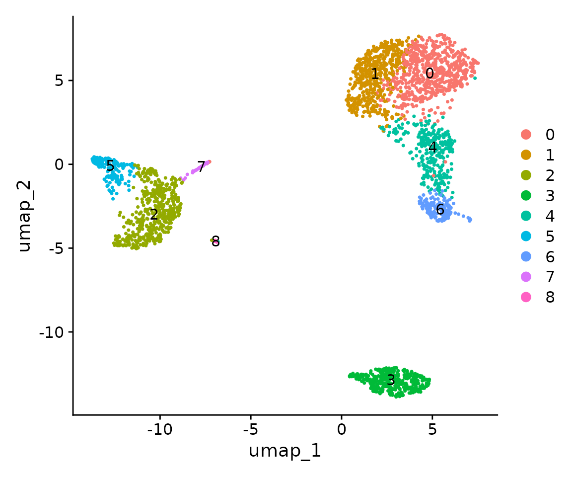

9. Annotate Cell Types

At this point, we have clusters named with numbers. But how do we determine what cell types these clusters represent, and how can we rename these numerical clusters with actual cell type names?

Cell annotation is a vast topic that we can’t cover comprehensively in this course. For now, we’ll focus on the most basic operations, with the opportunity to delve deeper later.

First, let’s visualize the expression of known marker genes to determine what cell types these clusters represent:

FeaturePlot(
  pbmc,
  features = c(
    "MS4A1", "GNLY", "CD3E",
    "CD8A", "CCR7", "CD14",
    "FCER1A", "FCGR3A", "PPBP"),
  order = TRUE)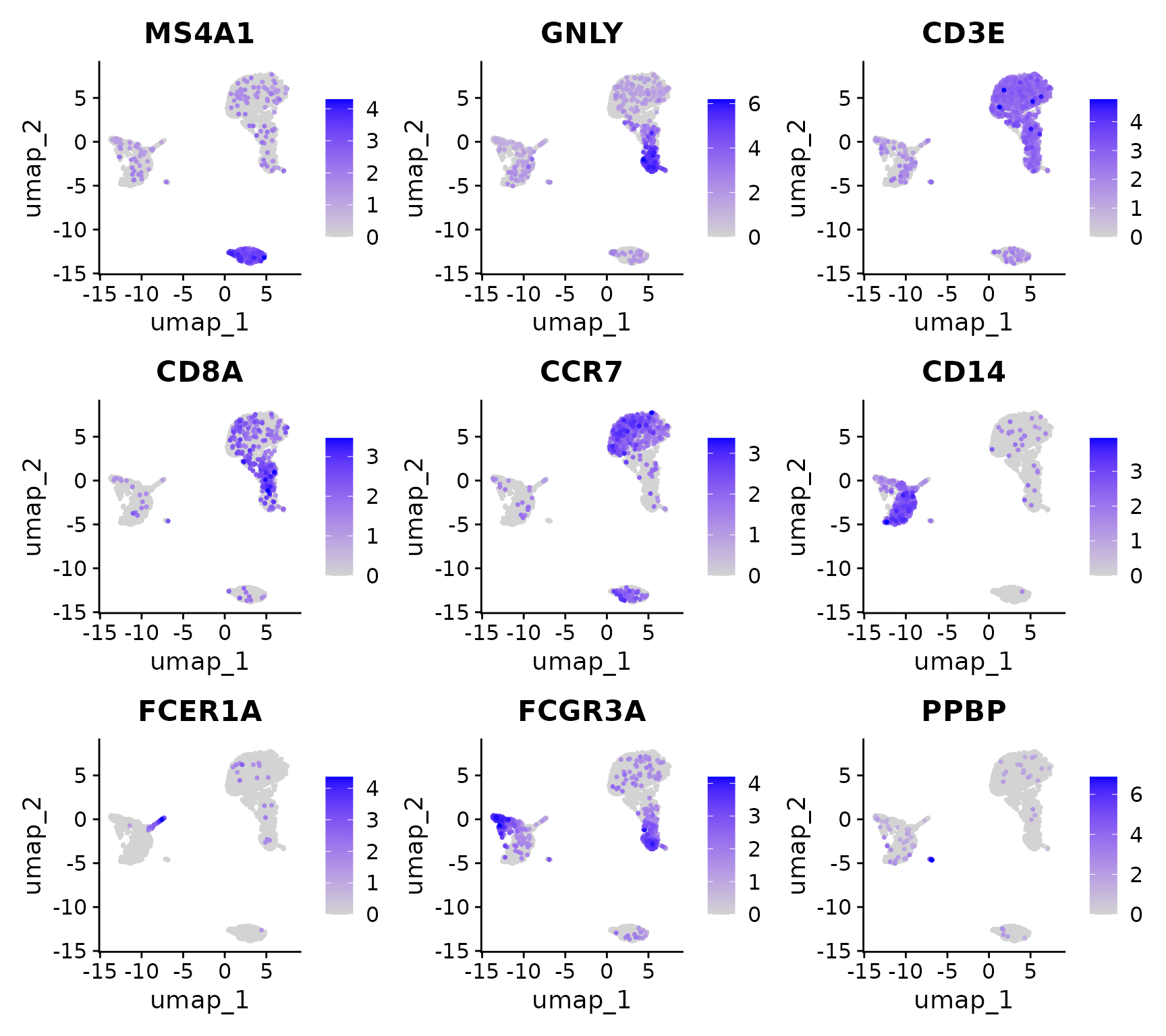

Now, let’s assign cell type labels based on marker gene expression. We’ll rename clusters 0-8 with our desired cell type names. This process utilizes the properties and techniques of factors that we learned earlier.

First, let’s examine the seurat_clusters column in meta.data:

head(pbmc$seurat_clusters)

## AAACATACAACCAC-1 AAACATTGAGCTAC-1 AAACATTGATCAGC-1 AAACCGTGCTTCCG-1 
##                0                3                0                5 
## AAACCGTGTATGCG-1 AAACGCACTGGTAC-1 
##                6                0 
## Levels: 0 1 2 3 4 5 6 7 8

We can see this is a factor. Note that we used $ directly on the Seurat object. We previously learned that @ is used to access specific object slots, while $ is more flexible, depending on how the developer defines it. For Seurat objects, since meta.data is one of the most commonly used tables, the developers set $ to directly access meta.data columns. Here, pbmc$seurat_clusters is equivalent to pbmc@meta.data$seurat_clusters.

Now, let’s copy the seurat_clusters column in meta.data to a new column called cluster:

pbmc$cluster <- pbmc$seurat_clusters
head(pbmc$cluster)

## AAACATACAACCAC-1 AAACATTGAGCTAC-1 AAACATTGATCAGC-1 AAACCGTGCTTCCG-1 
##                0                3                0                5 
## AAACCGTGTATGCG-1 AAACGCACTGGTAC-1 
##                6                0 
## Levels: 0 1 2 3 4 5 6 7 8

Since this is a factor, we can use the method we learned in the previous lesson to change the level names. We just need to change the current 0-8 to the corresponding cell types:

new.cluster.ids <- c("CD4 T Naive", "CD4 T Memory", "Mono CD14", "B cell", "CD8 T cell", "Mono FCGR3A", "NK cell", "DC", "Platelet")
levels(pbmc$cluster) <- new.cluster.ids
head(pbmc$cluster)

## AAACATACAACCAC-1 AAACATTGAGCTAC-1 AAACATTGATCAGC-1 AAACCGTGCTTCCG-1 
##      CD4 T Naive           B cell      CD4 T Naive      Mono FCGR3A 
## AAACCGTGTATGCG-1 AAACGCACTGGTAC-1 
##          NK cell      CD4 T Naive 
## 9 Levels: CD4 T Naive CD4 T Memory Mono CD14 B cell CD8 T cell ... Platelet

Let’s view the new annotation results:

DimPlot(pbmc, label = TRUE, group.by = "cluster")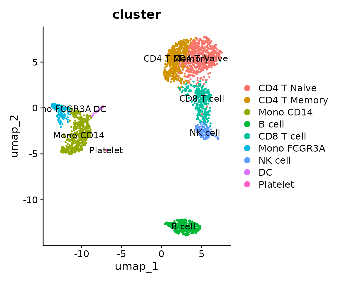

We can also sort the levels alphabetically:

pbmc$cluster <- factor(pbmc$cluster, levels = sort(levels(pbmc$cluster)))

Now, let’s visualize the final annotated UMAP:

DimPlot(pbmc, label = TRUE, group.by = "cluster")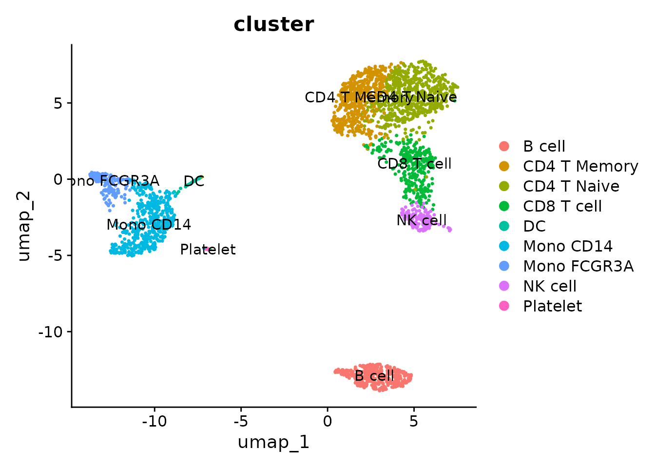

We can change the default idents, so we don’t need to specify the group.by parameter every time we use DimPlot:

Idents(pbmc) <- 'cluster'
DimPlot(pbmc, label = TRUE)

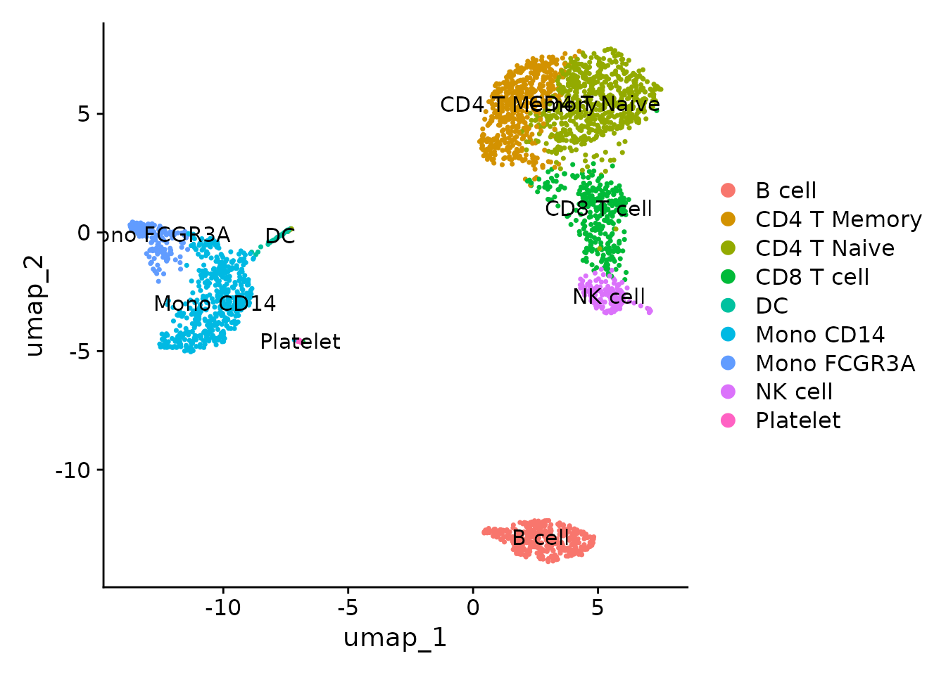
With this, we’ve completed the entire process from raw count matrix to annotated UMAP. This is a significant milestone in single-cell analysis. In the upcoming lessons, we’ll learn various visualization methods using the SeuratExtend package, as well as various advanced analyses.

Let’s save the current Seurat object as an RDS file:

# Create a new folder called 'rds' and save pbmc into it
dir.create("rds", showWarnings = FALSE)
saveRDS(pbmc, file = "rds/pbmc_annotated.rds")

Finally, let’s install SeuratExtend in preparation for the next lessons:

# If you haven't installed remotes yet:
if (!requireNamespace("remotes", quietly = TRUE)) {
    install.packages("remotes")
}
remotes::install_github("huayc09/SeuratExtend")

This concludes our basic single-cell analysis workflow with Seurat. In the next lessons, we’ll explore more advanced techniques and visualizations using SeuratExtend.

Yichao Hua

2024-11-29